
INTERNATIONAL PROGRAMME ON CHEMICAL SAFETY
ENVIRONMENTAL HEALTH CRITERIA 69
MAGNETIC FIELDS
This report contains the collective views of an international group of
experts and does not necessarily represent the decisions or the stated
policy of the United Nations Environment Programme, the International
Labour Organisation, or the World Health Organization.
Published under the joint sponsorship of
the United Nations Environment Programme,
the International Labour Organisation,
and the World Health Organization
World Health Orgnization
Geneva, 1987
The International Programme on Chemical Safety (IPCS) is a
joint venture of the United Nations Environment Programme, the
International Labour Organisation, and the World Health
Organization. The main objective of the IPCS is to carry out and
disseminate evaluations of the effects of chemicals on human health
and the quality of the environment. Supporting activities include
the development of epidemiological, experimental laboratory, and
risk-assessment methods that could produce internationally
comparable results, and the development of manpower in the field of
toxicology. Other activities carried out by the IPCS include the
development of know-how for coping with chemical accidents,
coordination of laboratory testing and epidemiological studies, and
promotion of research on the mechanisms of the biological action of
chemicals.
ISBN 92 4 154269 1
The World Health Organization welcomes requests for permission
to reproduce or translate its publications, in part or in full.
Applications and enquiries should be addressed to the Office of
Publications, World Health Organization, Geneva, Switzerland, which
will be glad to provide the latest information on any changes made
to the text, plans for new editions, and reprints and translations
already available.
(c) World Health Organization 1987
Publications of the World Health Organization enjoy copyright
protection in accordance with the provisions of Protocol 2 of the
Universal Copyright Convention. All rights reserved.
The designations employed and the presentation of the material
in this publication do not imply the expression of any opinion
whatsoever on the part of the Secretariat of the World Health
Organization concerning the legal status of any country, territory,
city or area or of its authorities, or concerning the delimitation
of its frontiers or boundaries.
The mention of specific companies or of certain manufacturers'
products does not imply that they are endorsed or recommended by the
World Health Organization in preference to others of a similar
nature that are not mentioned. Errors and omissions excepted, the
names of proprietary products are distinguished by initial capital
letters.
CONTENTS
ENVIRONMENTAL HEALTH CRITERIA FOR MAGNETIC FIELDS
PREFACE
1. SUMMARY, CONCLUSIONS, AND RECOMMENDATIONS FOR FURTHER STUDIES
1.1. Physical characteristics and dosimetric concepts
1.2. Natural background and man-made magnetic fields
1.3. Field measurement
1.4. Biological interactions
1.4.1. Interaction mechanisms
1.4.2. Biological effects of magnetic fields
1.5. Effects on man
1.5.1. Static fields
1.5.2. Time-varying fields
1.6. Exposure guidelines and standards
1.7. Protective measures
1.7.1. Cardiac pacemakers
1.7.2. Metallic implants
1.7.3. Hazards from loose paramagnetic objects
1.8. Recommendations for future research
2. PHYSICAL CHARACTERISTICS, DOSIMETRIC CONCEPTS, AND MEASUREMENT
2.1. Quantities and units
2.2. Dosimetric concepts
2.2.1. Static magnetic fields
2.2.2. Time-varying magnetic fields
2.3. Measurement of magnetic fields
2.3.1. Search coils
2.3.2. The Hall probe
2.3.3. Nuclear magnetic resonance probe
2.3.4. Personal dosimeters
3. NATURAL BACKGROUND AND MAN-MADE MAGNETIC FIELDS
3.1. Natural magnetic fields
3.2. Man-made sources
3.2.1. Magnetic fields in the home and public premises
3.2.1.1 Household appliances
3.2.1.2 Transmission lines
3.2.1.3 Transportation
3.2.1.4 Security systems
3.2.2. Magnetic fields in the work-place
3.2.2.1 Industrial processes
3.2.2.2 Energy technologies
3.2.2.3 Switching stations and power plants
3.2.2.4 Research facilities
3.2.2.5 Video display terminals
3.3. Magnetic fields in medical practice
3.3.1. Diagnosis, magnetic resonance imaging, and
metabolic studies
3.3.2. Therapy
4. MECHANISMS OF INTERACTION
4.1. Static magnetic fields
4.1.1. Electrodynamic and magnetohydrodynamic
interactions
4.1.2. Magnetomechanical effects
4.1.2.1 Orientation of diamagnetically
anisotropic macromolecules
4.1.2.2 Orientation of organisms with
permanent magnetic moments
4.1.2.3 Translation of substances in a
magnetic field gradient
4.1.3. Effects on electronic spin states
4.2. Time-varying magnetic fields
4.3. Other magnetic field interactions under study
4.3.1. Long-range cooperative phenomena in cell membranes
4.3.2. Localized interactions of external ELF
fields with cell membrane structures
5. EXPERIMENTAL DATA ON THE BIOLOGICAL EFFECTS OF STATIC MAGNETIC
FIELDS
5.1. Molecular interactions
5.2. Effects at the cell level
5.3. Effects on organs and tissues
5.4. Effects on the circulatory system
5.4.1. Linear relationship of induced flow potential and
magnetic field strength
5.4.2. Induced flow potentials and field orientation
5.4.3. Dependence of induced blood flow potentials on
animal size
5.4.4. Magnetohydrodynamic effects
5.4.5. Cardiac performance
5.5. Nervous system and behaviour
5.5.1. Excitation threshold of isolated neurons
5.5.2. Action potential amplitude and conduction velocity
in isolated neurons
5.5.3. Absolute and relative refractory periods of
isolated neurons
5.5.4. Effects of static magnetic fields on the
electroencephalogram
5.5.5. Behavioural effects
5.6. Visual system
5.7. Physiological regulation and circadian rhythms
5.8. Genetics, reproduction, and development
5.9. Conclusions
6. BIOLOGICAL EFFECTS OF TIME-VARYING MAGNETIC FIELDS
6.1. Visual system
6.2. Studies on nerve and muscle tissue
6.3. Animal behaviour
6.4. Cellular, tissue, and whole organism responses
6.5. Effects of pulsed magnetic fields on bone growth and
repair
6.6. Conclusions
7. HUMAN STUDIES
7.1. Studies on working populations
7.1.1. Workers exposed to static magnetic fields
7.1.2. Cancer epidemiological studies on workers exposed
to ELF electromagnetic fields
7.1.3. Conclusions
7.2. Epidemiological studies on the general population
7.3. Studies on human volunteers
8. HEALTH EFFECTS ASSESSMENT
8.1. Static magnetic fields
8.2. Time-varying magnetic fields
8.3. Conclusions
9. STANDARDS AND THEIR RATIONALES
9.1. Static magnetic fields
9.2. Time-varying magnetic fields
9.3. Magnetic resonance imaging guidelines
9.3.1. United Kingdom
9.3.2. USA
9.3.3. Federal Republic of Germany
9.3.4. Canada
10. PROTECTIVE MEASURES AND ANCILLARY HAZARDS
REFERENCES
WHO/IRPA TASK GROUP ON MAGNETIC FIELDS
Members
Dr V. Akimenko, A.N. Marzeev Research Institute of General and
Communal Hygiene, Kiev, USSR
Dr B. G. Bernardo, Philippine Atomic Energy Commission, Quezon
City, Philippines
Professor J. Bernhardt, Institute for Radiation Hygiene of the
Federal Health Office, Neuherberg, Federal Republic of
Germanya
Dr B. Bosnjakovic, Ministry of Housing, Planning and Environment,
Directorate of Radiation Protection, Stralenbescherming
Leidschendam, Netherlandsa
Mrs A. Duchêne, Commissariat à l'Energie Atomique, Département
de Protection Sanitaire, Fontenay-aux-Roses, Francea
Professor J. Dumansky, A. N. Marzeev Research Institute of
General and Communal Hygiene, Kiev, USSR
Professor M. Grandolfo, Radiation Laboratory, Higher Institute
of Health, Rome, Italya
Dr H. Jammet, Commissariat à l'Energie Atomique, Commissariat
à l'Energie Atomique, Institut de Protection et de Sûreté
Nucléaire, Fontenay-aux-Roses, France (Co-Chairman)a
Dr Y. A. Kholodov, Institute of Higher Nervous Activity and
Neurophysiology, Moscow, USSR
Professor B. Knave, Research Department, National Board of
Occupational Safety and Health, Solna, Swedena
Dr S. Mohanna, Radiation Protection Bureau, Environmental
Health Directorate, Ottawa, Ontario, Canada
Dr M. H. Repacholi, Royal Adelaide Hospital, Adelaide, South
Australia (Rapporteur)a
Dr R. D. Saunders, National Radiological Protection Board,
Chilton, Didcot, United Kingdom
Professor M. G. Shandala, A.N. Marzeev Research Institute of
General and Communal Hygiene, Kiev, USSR (Co-Chairman)
Mr J. Skvarca, National Direction of Environmental Quality,
Ministry of Health and Social Action, Buenos Aires,
Argentina
Members (contd.)
Mr D. Sliney, Laser Microwave Division, US Army Environmental
Hygiene Agency, Aberdeen Proving Ground, Maryland, USAa
Dr T.S. Tenforde, Lawrence Berkeley Laboratory, Biology and
Medicine Division, Berkeley, California, USA
Secretariat
Dr M. Swicord, Division of Diagnostic, Therapeutic and
Rehabilitative Technology, World Health Organization,
Geneva, Switzerland (WHO Consultant)
Dr P. J. Waight, Prevention of Environmental Pollution, World
Health Organization, Geneva, Switzerland (Secretary)
Observers
Dr Zh.I. Chernaya, A. N. Marzeev Research Institute of
General and Communal Hygiene, Kiev, USSR
Dr V. Voronin, Centre of International Projects, Moscow, USSR
Dr Z. Grigorevskaya, Centre of International Projects, Moscow,
USSR
Dr T. Lukina, Centre of International Projects, Moscow, USSR
---------------------------------------------------------------------------
a From the Committee on Non-Ionizing Radiation of the International
Radiation Protection Association.
NOTE TO READERS OF THE CRITERIA DOCUMENTS
Every effort has been made to present information in the
criteria documents as accurately as possible without unduly
delaying their publication. In the interest of all users of the
environmental health criteria documents, readers are kindly
requested to communicate any errors that may have occurred to the
Manager of the International Programme on Chemical Safety, World
Health Organization, Geneva, Switzerland, in order that they may be
included in corrigenda, which will appear in subsequent volumes.
* * *
PREFACE
The International Radiation Protection Association (IRPA)
initiated activities concerned with non-ionizing radiation by
forming a Working Group on Non-Ionizing Radiation in 1974. This
Working Group later became the International Non-Ionizing Radiation
Committee (IRPA/INIRC), at the IRPA meeting held in Paris in 1977.
The IRPA/INIRC reviews the scientific literature on non-ionizing
radiation and makes assessments of the health risks of human
exposure to such radiation. Based on the Environmental Health
Criteria Documents developed in conjunction with the International
Programme on Chemical Safety (IPCS), World Health Organization, the
IRPA/INIRC recommends guidelines on exposure limits, drafts codes
of safe practice, and works in conjunction with other international
organizations to promote safety and standardization in the non-
ionizing radiation field.
The first draft of this document was compiled by DR M.
REPACHOLI. An editorial group chaired by DR P. CZERSKI and
including DR V. AKIMENKO, PROFESSOR J. BERNHARDT, DR B.
BOSNJAKOVIC, MRS A. DUCHENE, PROFESSOR M. GRANDOLFO, DR M.
REPACHOLI, MR D. SLINEY, and DR T. TENFORDE met in Neuherberg in
May 1985 to develop the second draft. A small editorial group
consisting of DR P. CZERSKI, DR M. SWICORD, and DR P. WAIGHT met in
Geneva in April 1986 to collate and incorporate the comments
received from IPCS Focal Points and individual experts. The final
draft was then sent to WHO/IRPA Task Group members and formally
reviewed in Kiev, USSR, 30 June - 4 July 1986. Final scientific
editing of the document was completed by DR M. REPACHOLI, with the
assistance of DR M. SWICORD, in Geneva in July 1986. The
scientific assistance and helpful comments of DR T. TENFORDE, and
the permission to use his extensive literature files, are
gratefully acknowledged.
This document comprises a review of data of effects of magnetic
field exposure on biological systems, pertinent to the evaluation
of health risks for man. The purpose of the document is to provide
an overview of the known biological effects of magnetic fields, to
identify gaps in this knowledge so that direction for further
research can be given, and to provide information for health
authorities and regulatory agencies on the possible effects of
magnetic-field exposure on human health, so that guidance can be
given on the assessment of risks from occupational and general
population exposure.
Subjects reviewed include: the physical characteristics of
magnetic fields; measurement techniques; applications of magnetic
fields and sources of exposure; mechanisms of interaction;
biological effects; and guidance on the development of protective
measures, such as regulations or safe-use guidelines. Health
agencies and regulatory authorities are encouraged to set up and
develop programmes that ensure that the maximum benefit occurs with
the lowest exposure. It is hoped that this criteria document will
provide useful information for the development of national
protection measures against magnetic fields.
The WHO Regional Office for Europe prepared a publication
entitled Non-Ionizing Radiation Protection (WHO, 1982). A revised
and updated edition, completed in 1986, includes a section (5) on
Electrical and Magnetic Fields at Extremely Low Frequencies.
1. SUMMARY, CONCLUSIONS, AND RECOMMENDATIONS FOR FURTHER STUDIES
This document includes a detailed review and evaluation of data
on effects on human beings and other biological systems exposed to
static magnetic fields or to time-varying fields at extremely low
frequencies (ELF) of up to about 300 Hz. Data from the biological
effects of exposure to sinusoidally varying fields are mainly
concerned with effects in the range up to 20 Hz or at 50 and 60 Hz,
and only limited data are available on effects at higher
frequencies. Data on studies with higher frequencies and pulse
repetition rates, and non-sinusoidal waveforms have also been
considered, but radiofrequency magnetic fields in the frequency
range 100 kHz - 300 GHz have been excluded because these have been
treated in the Environmental Health Criteria 16: Radiofrequency and
microwaves (WHO, 1981).
Information for health authorities on the biological effects
and possible health effects of magnetic fields, is given to provide
guidance for the assessment of the occupational and public health
significance of exposure to magnetic fields and to indicate areas
that may be hazardous. Information on human exposure levels is
provided, which, on the basis of present knowledge, is considered
appropriate for the prevention of health hazards.
1.1. Physical Characteristics and Dosimetric Concepts
A magnetic field always exists when there is an electric
current flowing. A static magnetic field is formed in the case of
direct current, and a time-varying magnetic field is produced by
alternating current sources.
The fundamental vector quantities describing a magnetic field
are field strength, H (unit: A/m) and magnetic flux density, B
(unit: T, tesla). These quantities are related through B = µH,
where µ is the magnetic permeability of the medium.
The term "dosimetry" is used to quantify exposure. Present
understanding of interaction mechanisms is insufficient to develop
anything but preliminary dosimetric concepts for static or ELF
magnetic fields.
In practical radiation protection, it is useful to consider
static and time-varying magnetic fields separately. In the case of
static magnetic fields, protection limits tend to be stated
primarily in terms of the external field strength or magnetic flux
density and the duration of exposure. Since time-varying magnetic
fields induce eddy currents within the body, evaluation may be
based on the electric eddy current density (electric field
strength) in critical organs. Derived protection limits can then
be expressed as exposures to external magnetic fields, whereby
field strength, pulse shape (rise and decay time) and frequency,
orientation of the body, and duration of the exposure need to be
specified.
1.2. Natural Background and Man-Made Magnetic Fields
The natural magnetic field consists of a component originating
in the earth, acting as a permanent magnet, and several small
components with different spectral characteristics. At the
surface of the earth, the vertical component of the permanent field
is maximal at the magnetic poles, amounting to about 6.7 x 10⁻⁵ T
(67 µT), and is zero at the magnetic equator; the horizontal
component is maximal at the magnetic equator, amounting to about
3.3 x 10⁻⁵ T (33 µT), and is zero at the magnetic pole. The flux
density of the natural time-varying fields decreases from about
10-7 to 10-14 T when the frequency of the atmospheric
electromagnetic fields increases from about 0.1 Hz to 3 kHz.
The magnetic fields from man-made sources generally have higher
intensities than the naturally occurring fields. In the home and
public places, magnetic flux densities ranging from 0.03 µT to
30 µT are produced around household appliances, and up to 35 µT near
transmission lines (50 and 60 Hz), depending on the current carried
and the distance from the line. For magnetically-levitated
transportation systems, static magnetic fields of 6 - 60 mT are
expected in the region of a passenger's head. Security systems in
libraries and storehouses operate at frequencies of between 0.1 and
10 kHz and produce fields of up to about 1 mT.
Occupational exposure to magnetic fields is mainly encountered
in industrial processes involving high electric current equipment,
in certain new technologies for energy production and storage, and
in specialized research facilities. Around various types of
welding machines, furnaces, and induction heaters, the magnetic
flux densities at the operator location range from about 1 µT to
more than 10 mT, depending on the magnetic field frequency and the
distance from the coil. Compared to devices operating at high
frequencies, lower frequency induction heaters expose operators to
higher magnetic flux densities. At operator-accessible locations
in industries using electrolytic processes, the mean static field
level is about 5 - 10 mT.
In areas accessible to operations personnel in thermonuclear
magnetic fusion and magnetohydrodynamic generating systems, the
static magnetic field flux densities may reach 50 mT. Similar
field strengths occur near special research facilities, e.g.,
bubble chambers. Typical values for the magnetic flux density at
work-places near 50 or 60 Hz overhead transmission lines,
substations, and in power stations are up to 0.05 mT.
In medical practice, exposure to magnetic fields results mainly
from the use of magnetic resonance (MR) imaging or spectroscopy
methods for diagnostic purposes or from devices generating magnetic
fields for therapeutic purposes. In the MR-devices in use at
present, the patient is exposed to stationary magnetic fields with
intensities of up to 2 T and, during examinations, to time-varying
magnetic fields as high as 20 T/s. However, most patients are not
exposed to time-varying fields exceeding 1.5 T/s. The peak
exposure value for the patient caused by therapeutic magnetic
devices is of the order of 0.1 - 2.5 mT.
The increasing use of magnetic field-producing equipment in
industrial processes, research facilities, energy production and
distribution, new transportation technologies, consumer products
and medical practice, increases the possibility of human exposure
to magnetic fields. Although, up to now, both occupational and
general-population exposures to magnetic fields have generally been
at low levels, some new technologies, e.g., magnetically-levitated
trains, might result in exposure of the general population to
levels comparable with the highest ones in some working
environments. Thus, new technologies involving the production of
magnetic fields should be carefully evaluated with respect to
potential health risks.
1.3. Field Measurement
In order to adequately characterize a magnetic field, the
magnitude, frequency, and direction of the field must be
determined. The spatial properties of the field can become
complicated by time-varying changes in the direction of the
resultant magnetic field vector. For example, for a circularly
polarized field, the magnetic vector describes an ellipse during
the course of a cycle and does not reach zero magnitude.
Principles of calculation and measurement of these fields are
outlined.
A human or animal body located in a magnetic field causes
virtually no perturbation of the field. A time-varying magnetic
field induces electric currents in the exposed body. The factors
affecting the magnitude of the induced currents are discussed
below.
1.4. Biological Interactions
The following topics are summarized: the present state of
knowledge on the mechanisms by which magnetic fields interact with
living systems, and the biological effects of these fields. On the
basis of available information, the areas of future research that
appear to hold the greatest potential for elucidating some poorly
understood aspects of magnetic field interactions with biological
systems are given at the end of this section.
1.4.1. Interaction mechanisms
There are three established physical mechanisms through which
static and ELF magnetic fields interact with living matter:
A. Magnetic induction
This mechanism is relevant to both static and time-varying
fields, and originates through the following types of interaction:
(a) Electrodynamic interactions with moving electrolytes
Both static and time-varying fields exert Lorentz forces on
moving ionic charge carriers, and thereby give rise to induced
electric fields and currents. This interaction is the basis of
magnetically-induced blood flow potentials that have been studied
with both static and time-varying ELF fields. It is also the
physical basis of the weak induced potentials that provide sensory
directional cues to elasmobranch fish as they swim through the
static geomagnetic field.
(b) Faraday currents
Time-varying magnetic fields induce currents in living tissues
in accordance with the Faraday law of induction. Available evidence
suggests that this mechanism may underlie the visuosensory
stimulation that produces magnetophosphenes and other effects on
electrically excitable tissues. In addition, indirect evidence
suggests that rapidly time-varying magnetic fields may exert
effects on a variety of cellular and tissue systems by inducing
local currents that exceed the naturally occurring levels. This
effect may be the basis for the wide spectrum of biological
perturbations that have been observed with pulsed magnetic fields,
such as those used clinically for bone fracture reunion.
B. Magnetomechanical effects
The two types of mechanical effects that a static magnetic
field exerts on biological objects are:
(a) Magneto-orientation
In a uniform static field, both diamagnetic and para-magnetic
molecules experience a torque, which tends to orientate them in a
configuration that minimizes their free energy within the field.
This effect has been well studied for assemblies of diamagnetic
macromolecules with differing magnetic susceptibilities along the
principal axes of symmetry. Included in this class of
macromolecules are the arrays of photopigments in retinal rod disc
membranes.
(b) Magnetomechanical translation
Spatial gradients of static magnetic fields produce a net force
on paramagnetic and ferromagnetic materials that leads to
translational motion. Because of the limited amount of magnetic
material in most living objects, the influence of this effect on
biological functions is negligible.
C. Electronic interactions
Certain classes of chemical reactions involve radical electron
intermediate states in which interactions with a static magnetic
field produce an effect on electronic spin states. It is possible,
that the usual lifetime of biologically relevant electron
intermediate states is sufficiently short that magnetic field
interactions exert only a small, and perhaps negligible, influence
on the yield of chemical reaction products.
In addition to the mechanisms of magnetic field interactions
for which there is direct experimental evidence, several other
mechanisms have been proposed, on theoretical grounds, in an effort
to explain various biological effects that have been reported to
occur in static and ELF fields of very low intensity. However, it
must be emphasized, that many proposed mechanisms have not been
subjected to direct experimental tests.
1.4.2. Biological effects of magnetic fields
Some organisms possess sensitivity to static magnetic fields
with low intensities comparable to that of the geomagnetic field
(about 50 µT). Phenomena for which there is substantial
experimental evidence of sensitivity to the earth's field include:
(a) direction finding by elasmobranch fish (shark, skate,
and ray);
(b) orientation and swimming direction of magnetotactic
bacteria;
(c) kinetic movements of molluscs;
(d) migratory patterns of birds; and
(e) waggle dance of bees.
In addition, a number of in vitro studies have been made of
magnetic orientation in assemblies of macromolecules, including
retinal rod outer segments, muscle fibres, photosynthetic systems
(chloroplast grana, photosynthetic bacteria, and Chlorella cells),
halobacteria purple membranes, and various synthetic liquid
crystals and gels. As discussed in the preceding summary of
mechanisms of magnetic field interaction, certain classes of
chemical reactions that involve a radical electron intermediate
state may also be sensitive to static magnetic fields of moderate
intensity (< 10 mT).
The available experimental information on the response of
organisms, including land-dwelling mammalian species, to static and
ELF magnetic fields indicates that three biological effects can be
regarded as established phenomena:
(a) the induction of electrical potentials within the
circulatory system;
(b) magnetophosphene induction by pulsed and ELF magnetic
fields with a time rate of change exceeding 1.3 T/s
or sinusoidal fields of 15 - 60 Hz and field
strengths ranging from 2 to 10 mT (frequency
dependent); and
(c) the induction by time-varying fields of a wide
variety of cellular and tissue alterations, when the
induced current density exceeds 10 mA/m2; many of
these effects appear to be the consequence of
interactions with cell membrane components.
For static magnetic fields with flux densities of less than 2
T, there exists a body of experimental data that indicates the
absence of irreversible effects on many developmental,
behavioural, and physiological parameters in higher organisms.
Broadly summarized, available evidence suggests that the following
9 classes of biological functions are not significantly affected by
static magnetic fields at levels up to 2 T:
(a) cell growth;
(b) reproduction;
(c) pre- and post-natal development;
(d) bioelectric activity of isolated neurons;
(e) behaviour;
(f) cardiovascular functions (acute exposures);
(g) the blood-forming system and blood;
(h) immune system functions;
(i) physiological regulation and circadian rhythms.
For time-varying magnetic fields in the ELF frequency range,
few systematic studies have been carried out to define the
threshold field characteristics for producing significant
perturbations of biological functions. Nevertheless, available
evidence suggests that ELF magnetic fields must induce current
densities in tissues and extracellular fluids that exceed
10 mA/m2, in order to produce significant alterations in the
development, physiology, and behaviour of intact higher organisms.
In in vitro studies, various phenomena have been reported in the
1 - 10 mA/m2 range, but their health significance has not been
determined. However, it should be noted that therapeutic
applications of magnetic fields make use of this range.
1.5. Effects on Man
1.5.1. Static fields
Studies on workers involved in the manufacture of permanent
magnets in the USSR indicated various subjective symptoms and
functional disturbances including irritability, fatigue, headache,
loss of appetite, bradycardia, tachycardia, decreased blood
pressure, altered EEG, itching, burning, and numbness. However,
lack of any statistical analysis or assessment of the impact of
physical or chemical hazards in the working environment
significantly reduces the value of these reports. Although the
studies are inconclusive, they suggest that, if long-term effects
occur, they are very subtle, since no cumulative gross effects are
evident.
Recent epidemiological surveys in the USA have failed to reveal
any significant health effects associated with long-term exposure
to static magnetic fields. A study of the health data on 320
workers in plants using large electrolytic cells for chemical
separation processes, where the average static field level in the
work environment was 7.6 mT and the maximum field was 14.6 mT,
indicated slight changes in white blood cell picture (still within
the normal range) in the exposed group compared with the 186
controls. None of the observed changes in blood pressure or blood
parameters was considered indicative of a significant adverse
effect associated with magnetic field exposure.
The prevalence of disease among 792 workers at the US National
Accelerator Laboratories, who were exposed occupationally to static
magnetic fields, was compared with that in a control group
consisting of 792 unexposed workers matched for age, race, and
socioeconomic status. The range of magnetic field exposures was
from 0.5 mT for long durations to 2 T for periods of several hours.
No significant increase or decrease in the prevalence of 19
categories of disease was observed in the exposed group relative to
the controls.
Workers exposed to large static magnetic fields in the
aluminium industry were reported to have an elevated leukaemia
mortality rate. Although these studies suggest an increased cancer
risk for persons directly involved in aluminium production, there
is no clear evidence, at present, indicating the responsible
carcinogenic factors within the work environment.
It can be concluded that available knowledge indicates the
absence of any adverse effects on human health due to exposure to
static magnetic fields up to 2 T. It is not possible to make any
definitive statements about safety or hazard associated with
exposure to fields above 2 T. From theoretical considerations and
some experimental data, it could be inferred that short-term
exposure to static fields above 5 T may produce significant
detrimental effects on health.
1.5.2. Time-varying fields
Time-varying magnetic fields generate internal electric
currents. For example, 3 T/s can induce current densities of about
30 µA/m2 around the perimeter of the human head. Induced electric
current densities can be used as the decisive parameter in the
assessment of the biological effects at the cellular level.
In terms of a health risk assessment, it is difficult to
correlate the internal tissue current densities with the external
magnetic field strength. However, assuming worst-case conditions,
it is possible to calculate, at least within one order of
magnitude, the magnetic flux density that would produce potentially
hazardous current densities in tissues. The following statements
can be made on induced current density ranges and correlated
magnetic flux densities of a sinusoidal homogeneous field, which
produce biological effects from whole-body exposure:
(a) Between 1 and 10 mA/m2 (induced by magnetic fields
above 0.5 - 5 mT at 50/60 Hz, or 10 - 100 mT at 3
Hz), minor biological effects have been reported.
(b) Between 10 and 100 mA/m2 (above 5 - 50 mT at 50/60 Hz
or 100 - 1000 mT at 3 Hz), there are well established
effects, including visual and nervous system
effects. Facilitation of bone fracture reunion has
been reported.
(c) Between 100 and 1000 mA/m2 (above 50 - 500 mT at
50/60 Hz or 1 - 10 T at 3 Hz), stimulation of
excitable tissue is observed and there are possible
health hazards.
(d) above 1000 mA/m2 (greater than 500 mT at 50/60 Hz or
10 T at 3 Hz), extra systoles and ventricular
fibrillation, i.e., acute health hazards, have been
established.
For non-sinusoidal waveforms that have short duration pulses,
the time rate of change of the magnetic flux density must be
specified. In analysing certain biological effects, especially the
stimulation of excitable tissue, the peak current density values
are more relevant than root mean square (rms) values. In addition,
non-homogeneous magnetic fields must be considered, since high
field gradients exist near strong magnetic field sources. The
induction loops in extremities are usually smaller than those in
the whole body, so higher magnetic field strengths are tolerable
for extremities than for the whole body.
Several laboratory studies have been conducted with human
subjects exposed to sinusoidally time-varying magnetic fields with
frequencies in the ELF range. None of these investigations has
revealed adverse clinical or psychological changes in the exposed
subjects. The strongest field used in these studies with human
volunteers was a 5-mT, 50-Hz field to which subjects were exposed
for 4 h.
Several recent epidemiological reports present preliminary data
indicative of an increase in the incidence of cancer among
children, adults, and occupational groups. In other
epidemiological studies in the USA, no apparent increases in
genetic defects or abnormal pregnancies were reported. The studies
that show an excess of cancers in children and adults suggest an
association with exposure to very weak (10-7 - 10-6 T) 50 or 60 Hz
magnetic fields that are of a magnitude commonly found in the
environment. These associations cannot be satisfactorily explained
by the available theoretical basis for carcinogenesis by ELF
electromagnetic fields. The preliminary nature of the
epidemiological evidence, and the relatively small increment in
reported incidence, suggest that, although these epidemiological
data cannot be dismissed, there must be considerable further study
before they can be accepted.
From the available data on human exposure to time-varying
magnetic fields, it can be concluded that induced current densities
below 10 mA/m2 have not been shown to produce any significant
biological effects. In the range of 10 - 100 mA/m2 (from fields
higher than 5 - 50 mT at 50/60 Hz), biological effects have been
established, but these induced current densities from short-term
exposure (few hours) may cause minor transient effects on health.
The health consequences of exposure to these levels for many
hours, days, or weeks are not known at present. Above 100 mA/m2
(greater than 50 mT at 50/60 Hz), various stimulation thresholds
are exceeded and hazards to health may occur.
1.6. Exposure Guidelines and Standards
Standards or guidelines limiting human exposure to static ELF
magnetic fields have been developed in a few countries. Of
particular interest is the increasing tendency of countries to
limit magnetic field exposure from particular devices (e.g.,
magnetic resonance diagnostic techniques). Details of these
standards and guidelines are given in section 9 of the document.
1.7. Protective Measures
Two aspects of magnetic field safety that deserve special
attention are the potential influence of these fields on the
functioning of electronic devices, and the risk of injury due to
the large forces exerted on ferromagnetic objects in strong static
magnetic field gradients. Of particular concern is the malfunction
of cardiac pacemakers and the displacement of aneurysm clips and
prosthetic devices.
1.7.1. Cardiac pacemakers
Both static and time-varying magnetic fields can interfere with
the proper functioning of modern demand pacemakers. Some
pacemakers may revert from a synchronous to an asynchronous mode of
operation in time-varying fields with time rates of change above
approximately 40 mT/s. Certain pacemaker models also exhibit
abnormal operation due to closure of a reed relay switch in static
magnetic fields that exceed 1.7 - 4.7 mT. Magnetic fields can also
affect the functioning of other medical electronic monitoring
devices, such as EEG and ECG equipment.
1.7.2. Metallic implants
The sensitivity of implanted surgical devices to magnetic
fields is dependent on their alloy composition. A large number of
metallic devices such as intrauterine devices, surgical clips,
prostheses, infusion needles, and catheters may have a significant
torque exerted on them by intense magnetic field gradients. This
may result in their displacement and produce serious consequences.
All persons entering magnetic field environments should be screened
carefully and, if necessary, prohibited from access.
1.7.3. Hazards from loose paramagnetic objects
Depending on the weight and shape of a paramagnetic object
subject to an intense magnetic field, it can become a missile with
high momentum. Care should be taken to exclude such objects as,
for example, scissors, scalpels, and handtools from the vicinity of
strong magnetic field sources.
1.8. Recommendations for Future Research
On the basis of present knowledge of magnetic field bioeffects,
several key areas of future research can be identified as being
essential for achieving a comprehensive understanding of the
biological consequences of exposure to these fields. No attempt
has been made to list all possible research areas. Instead,
emphasis has been placed on areas considered to have an impact on
health hazard assessment.
For static magnetic fields, there is a clear need for
additional studies in the following areas, in each of which the
available information is either inadequate or contradictory:
(a) studies on functional alterations in the cardiovascular
and central nervous system, where magnetic field
interactions have previously been observed; particular
emphasis should be placed on the effects of long-term
exposures;
(b) sensitivity of enzyme reactions that involve radical
intermediate states, which may be an important issue in
long-term occupational exposures;
(c) cellular, tissue, and animal responses to static fields
above 2 T, as proposed for use in clinical MR
spectroscopy.
For time-varying magnetic fields with repetition frequencies in
the ELF range, key areas of future research can also be recommended
on the basis of available information:
(a) Comprehensive epidemiological studies should be
carried out to resolve the issue of whether an
elevated risk of leukaemia and other forms of cancer
is associated with occupational and residential
exposure to ELF fields. These studies should include
the use of appropriate techniques for the assessment
of field exposure parameters (e.g., the use of
miniature personal dosimeters). Relevant research
with cellular and animal systems should also be
conducted in an effort to elucidate interaction
mechanisms of ELF fields that could lead to an
elevated cancer risk.
(b) Studies on the response of developing embryonic and
fetal systems, and other cell and tissue systems that
have been identified as being responsive to ELF
magnetic fields, should be continued with particular
focus on effects mediated via interactions with cell
membranes.
(c) Studies are needed on the effects of low levels of
induced current density (< 100 mA/m2) on nerve tissue.
2. PHYSICAL CHARACTERISTICS, DOSIMETRIC CONCEPTS, AND MEASUREMENT
Just as an electric field is always linked with an electric
charge, a magnetic field always appears when electric current
flows. A magnetic field can be illustrated by lines of force. A
static magnetic field is formed in the case of direct current,
whereas a time-varying magnetic field is induced by alternating
current sources.
The electric (E) and magnetic (H) fields that exist near
sources of electromagnetic fields must be considered separately,
because the very long wavelength (thousands of kilometres)
characteristic of extremely low frequencies (ELF) means that
measurements are made in the non-radiating near field. The E and H
fields do not have the same constant relationship that exists in
the far field of a radiating source.
A description of the physical characteristics of static and ELF
magnetic fields has been given by Grandolfo & Vecchia (1985a). An
animal or human body does not appreciably distort a magnetic field.
Time-varying magnetic fields induce currents within the body. The
magnitude of these internal currents is determined by the radius of
the current path, the frequency of the magnetic field and its
intensity at the location within the body. Unlike the electric
field for which the internal field strength is many orders of
magnitude less than that of the external field, the magnetic field
strength is virtually the same outside the body as within. The
magnetically-induced electric field strengths and corresponding
current density are greatest at the periphery of the body where the
conducting paths are longest, whereas microscopic current loops
anywhere within the body would have extremely small current
densities. The magnitude of the current density is also influenced
by tissue conductivity where the exact paths of the current flow
depend in a complicated way on the conducting properties of the
various tissues.
2.1. Quantities and Units
The quantities, units, and symbols used in describing magnetic
fields are given in Table 1.
The fundamental vector quantities describing a magnetic field
are the field strength (H) and the magnetic flux density (B) (or
equivalently, the magnetic induction).
The magnetic field strength (H) is the force with which the
field acts on an element of current situated at a particular
point. The value of H is measured in ampere per metre (A/m). The
trajectories of the motion of an element of current (or the
orientations of an elementary magnet) in a magnetic field are
called the magnetic lines of force.
Table 1. Magnetic field quantities and units in the SI
System
-----------------------------------------------------------
Quantity Symbol Unit
-----------------------------------------------------------
Frequency f hertz (Hz)
Current I ampere (A)
Current density J ampere per square metre
(A/m2)
Magnetic field strength H ampere per metre (A/m)
Magnetic flux PHI weber (Wb) = Vs
Magnetic flux density B tesla (T) = Wb/m2
Permeability µ henry per metre (H/m)
Permeability of vacuum µo µo = 1.257 x 10⁻⁶ H/m
Time t seconds (s)
-----------------------------------------------------------
As in the case of electric fields, single-phase and three-phase
magnetic fields can be defined: the field at any point may be
described in terms of its time-varying magnitude and invariant
direction (single-phase), or by the field ellipse, i.e., the
magnitude and direction of the major and minor semi-axes (three
phase).
The magnetic flux density (B), rather than the magnetic field
strength, (H = B/µ), is used to describe the magnetic field
generated by currents in the conductors of transmission lines and
substations. Thus, the magnetic field is defined as a vector field
of magnetic flux density B (B-field). The value of µ (the magnetic
permeability) is determined by the properties of the medium, and,
for most biological material is equal to µo, the value of the
permeability of free space (air). Thus, for biological materials
the values of B and H are related by a constant (µo).
Before the introduction of the International System of units
(SI), the use of the CGS system (based on the three independent
quantities: length (cm), mass (g) and time (s)) was customary. SI
is based on seven independent quantities: length (m), mass (g),
time (s), electric current (A), thermodynamic temperature (K),
luminous intensity (cd), and amount of substance (mol). The
equations describing the electromagnetic phenomena are equivalent
but not identical in the SI and the CGS systems. For an
electromagnetic field, only the first four of the seven quantities
mentioned above, are relevant. The CGS unit of magnetic field
strength is the oersted and that of the magnetic induction is the
gauss.
In the CGS system, µo is a dimensionless quantity equal to
unity, and as a result, for biological materials, B can be set
equal to H, as a close approximation. This convention has been
used extensively in the biological literature, where many authors
have used B and H as interchangeable quantities. Thus, many
publications contain equations that are appropriate for use only
with the CGS system of units since the permeability of free space,
µo, has been omitted.
The SI system has now been universally accepted. The CGS
system is obsolete and should not be used.
In addition, the term gamma is used and is equal to 1 nanotesla
(10-9 tesla). For convenience, the conversion factors relating the
various quantities used in laboratory practice are given in Table 2.
Table 2. Conversion factors for units
---------------------------------------------------------------------------
To
obtain T = Wb/m2 G gamma A/m Oe
-----------
To convert
---------------------------------------------------------------------------
T = Wb/m2 1 104 109 7.96 x 10⁵ 104
G 10-4 1 105 79.6 1
gamma 10-9 10-5 1 7.96 x 10⁻⁴ 10-5
A/m 1.256 x 10⁻⁶ 1.256 x 10⁻² 1256 1 1.256 x 10⁻²
Oe 10-4 1 105 79.6 1
---------------------------------------------------------------------------
Symbols: T = tesla
Wb = weber
G = gauss
A = ampere
m = metre
Oe = oersted
For a more complete inventory and discussion of quantities and
units, the reader is referred to a report of the IRPA/International
Non-Ionizing Radiation Committee entitled "Review of Concepts,
quantities, units, and terminology for non-ionizing radiation
protection" (IRPA, 1985).
2.2. Dosimetric Concepts
In its broadest sense, the term "dosimetry" is used to quantify
exposure to radiation. Quantitative descriptions of exposure, for
the purpose of formulating protection standards and exposure
limits, require the use of appropriate quantities. "Appropriate"
means that the quantities should represent, as far as possible, the
physical processes that are closely linked to the biological
effects of the fields. Since our knowledge of interaction
mechanisms is incomplete, exposure conditions are often quantified
in terms of the unperturbed external magnetic field strength and
the duration of exposure.
The known physical mechanisms by which magnetic fields interact
with living matter are described in section 4. Some factors
affecting the interaction of fields with organisms are summarized
in Table 3. To fully assess the data obtained in bioeffects
research, exposure conditions must be well controlled and measured.
In this case, the "dosimetry" in bioeffects research with magnetic
fields is very complex, since all relevant factors must be taken
into account. The accuracy and sophistication of radiation
protection dosimetry must be related to the conditions and actual
or potential adverse consequences of exposure to magnetic fields.
In practical radiation protection, it is useful to consider
static and time-varying magnetic fields separately.
Table 3. Factors affecting interaction of magnetic fields
---------------------------------------------------------------
Parameters of the magnetic field source
1. Frequency
2. Modulation (Pulse, AM, FM), rise and decay times (dB/dt)
3. Polarisation
4. Field strength
5. Field pattern (uniformity)
6. Surrounding material properties
Parameters related to exposure
1. Tissue properties (conductivity, anisotropy, permeability)
2. Size, geometry
3. Orientation relative to polarization
4. Mode of exposure (partial; whole body)
Extraneous factors
1. Metal implants (ferromagnetic)
2. Metal objects in the field
3. Drugs (medications)
4. Chemical pollutants
---------------------------------------------------------------
2.2.1. Static magnetic fields
In the assessment of exposure to static magnetic fields for
practical radiation protection purposes, the appropriate quantities
are less well defined. Protection limits tend to be stated in
terms of the external field strength and the duration of exposure,
where the integrated product of field and exposure time could be
considered as a measure of exposure. However, at present, there
is no biological basis for choosing this dosimetric concept.
Further development of dosimetric concepts and their theoretical
and experimental basis is required.
2.2.2. Time-varying magnetic fields
In evaluating human exposure to time-varying magnetic fields of
frequencies between about 10 Hz and 100 kHz, the electric eddy
current density can be employed as the decisive parameter in
assessment of the biological effects at the cellular level
(Bernhardt, 1979, 1985, 1986; Czerski, 1986; Tenforde, 1986a).
Field strength and eddy current density are related by the specific
conductivity of the medium.
By comparing the current densities, it may be possible to
predict effects in human beings from those found in studies on
animal and isolated cells. In this context, it is irrelevant
whether the current density surrounding a cell is introduced into
the body through electrodes or induced in the body by external
magnetic fields. However, the current paths within the body may be
different.
The evaluation of human exposure using current densities is
based primarily on a concept of "dose" to the critical organs.
Although this assumption is based on the most likely hypothesis,
this mechanism of energy absorption in tissues should not be
considered to the exclusion of all others. The parameters of
internal field strength and duration should also be taken into
account. Basic protection limits can be expressed in permissible
current densities; derived protection limits can be expressed as
exposures to external magnetic fields, where field strength,
frequency, orientation of the body, and duration of exposure need
to be specified. Refinements may include field gradient values,
partial body exposure, etc. Induced eddy currents in organs cannot
be measured, at present, under any practical conditions.
Therefore, the only protection quantities that can be used to
assess exposure to time-varying magnetic fields are the field
strength distribution in time and space.
2.3. Measurement of Magnetic Fields
During the last thirty years, the measurement of magnetic
fields has undergone considerable development. Progress in
techniques has made it possible to develop new methods of
measurement as well as to improve old ones. Some of the incentive
for considerable development in magnetic measurement techniques has
arisen because of the necessity to accurately measure magnetic
fields that often vary in both space and time in large particle
accelerators. The rapid development of plasma physics as well as
that of astronautics has created new demands for magnetic field
measurements.
A description of the most common measuring techniques follows,
together with a comparison of their advantages and limitations.
Further details can be found in Williamson & Kaufman (1981),
Grandolfo & Vecchia (1985a), and Stuchly (1986).
The two most popular types of magnetic field probes are a
shielded coil and a Hall-probe. Most of the commercially available
magnetic field meters use one of them. Recently, in addition to
Hall probes, other semiconductor devices, namely bipolar
transistors and FET transistors, have been proposed as magnetic
field sensors. They offer some advantages over Hall probes, such
as higher sensitivity, greater spatial resolution, and broader
frequency response.
For measurements of very weak magnetic fields, such as those
produced by endogeneous currents in biological systems, other
sensors are used. These include fluxgates, optically pumped
magnetometers, magnetostrictive sensors with optical fibres, and
superconducting quantum interference devices (SQUIDS). These
devices are rather specialized and expensive and are not normally
used for the measurement of extraneous fields in biomedical
applications (Stuchly, 1986).
2.3.1. Search coils
The operating principle of a coil B-field probe can be
explained by considering a closed loop of a conductor with area A
immersed in a quasi-static, uniform magnetic field of flux density
B, and angular frequency omega(= 2 pi f), as shown in Fig. 1 (Conti,
1985).
An electromotive force (EMF) is induced in the loop (and a
current (I) will flow) as a consequence of changes in the magnetic
flux PHI(B) through the area A, in accordance with the following
law:
d
EMF = -- PHI(B) (1)
dt
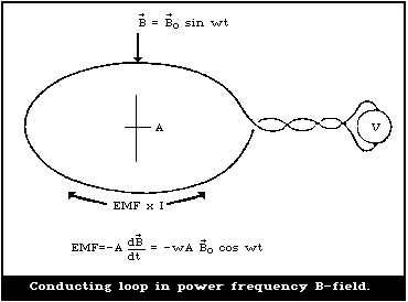 If the vector B = Bo sin omega t is assumed to be uniform and
to have its direction perpendicular to the plane of the loop, the
EMF is given by the following relationship:
d
EMF = - -- (A Bosin omega t) = omega Bo A cos omega t (2)
dt
Equation (2) shows that measurement of induced electromotive
force provides a measure of the B-field strength.
For a loop of many turns, the EMF given by Equation (2) will
develop over each turn and the voltage (V) will increase
accordingly. The induced current has been assumed to be so small
that the opposing B-field generated by I can be ignored.
There is no theoretical limit on the frequency of operation of
coils as sensors, except for the loop size. In practice, factors
such as the electric field perturbation and the pick up by the
leads connecting the loop to the metering device require
modifications of the sensor design.
A single coil has a directional spatial response
characteristic, and has to be rotated to obtain a maximum reading
to determine the actual magnitude and direction of the field.
Alternatively, a probe consisting of three mutually perpendicular
coils can be designed.
2.3.2. The Hall probe
The most commonly used method in field mapping is the Hall
probe. When a strip of conducting material is placed along the Ox
axis in a coordinate system Oxyz, with a current I running in the
direction Ox while a magnetic field B is applied in the direction
Oy at right angles to the surface of the strip, a potential
difference appears in the direction Oz between the two sides of the
strip.
The Hall effect can be explained as the result of the action
exerted on the charge carriers by the magnetic field, which forces
them sideways in the strip. Thus, electric charges appear on the
sides of the strip and, as a result, a transverse Hall electric
field is created.
Several factors set limits on the accuracy obtainable, the most
serious being the temperature coefficient of the Hall voltage.
Another complication can be that of the planar Hall effect, which
makes the measurement of a weak field component normal to the plane
of the Hall plate problematical, when a strong field component is
present parallel to this plane. Many possible remedies have been
proposed, but they are all relatively difficult to apply. Last,
but not least, is the problem of the representation of the
calibration curve since the Hall coefficient varies with the
magnetic field.
The measurement of the Hall voltage sets a limit of about 0.1
mT on the sensitivity and resolution of the measurement, if
conventional direct current excitation is applied to the probe.
The sensitivity can be improved considerably by using alternating
current excitation. Higher accuracy at low field strengths can be
achieved by using synchronous detection techniques for the
measurement of the Hall voltage.
Hall plates are usually calibrated in a magnet in which the
field is measured simultaneously using a nuclear magnetic resonance
probe. A well designed Hall-probe assembly can be calibrated to an
accuracy of 0.01% (Germain, 1963).
2.3.3. Nuclear magnetic resonance probe
Nuclear magnetic resonance (NMR) is the classical method of
measuring the absolute value of a magnetic field.
If a charged particle possessing an angular momentum vector, J,
is placed in a constant magnetic field B, the magnetic moment, u,
of the particle becomes orientated with respect to B. The vectors
J and u are proportional, u = gamma J where gamma is the
gyromagnetic ratio of the particle considered. In a quantum
mechanics description, this orientation can only be such that the
component of J along B is equal to mh/2pi, where m = ±(I - k),
I is the spin of the particle, and k is an integer smaller or
equal to I. Thus, m can take on several discrete values, each
giving a different orientation for J and u. Each of these
orientations of u in the magnetic field corresponds with a
different energy level, where these levels differ in energy by
DELTA E = B gamma h/2pi.
If a sample containing a large number of particles, either
electrons or protons, is irradiated with photons of the right
frequency, upsilono, such that h upsilono = DELTA E, an exchange of
energy occurs. As a result of photon absorption, particles in the
sample jump from the lower to the higher energy level. The
principle of the NMR measurement technique is to determine the
resonant frequency of the test specimen in the magnetic field to be
measured. It is an absolute measurement that can be made with very
great accuracy. The measuring range of this method is from about
10-2 to 10 T, without definite limits.
In field measurements using the proton magnetic resonance
method, an accuracy of 10-4 is easily obtained with simple
apparatus and an accuracy of 10-6 can be reached with extensive
precautions and refined equipment.
The inherent shortcoming of the NMR method is its limitation
to fields with a low gradient and the lack of information about
the field direction.
2.3.4. Personal dosimeters
A personal dosimeter suitable for monitoring exposures to
static and time-varying magnetic fields has been developed by
Fujita & Tenforde (1982). Using thin-film Hall sensors that record
magnetic induction (B) along three orthogonal axes, the time rate
of change of the magnetic induction (dB/dt) is determined for
values of B recorded during consecutive sampling intervals. The
parameters stored by the dosimeter include the average and peak
values of B and dB/dt during a preset time interval, and the number
of times that specified threshold levels of these parameters are
exceeded. An audible alarm sounds when B or dB/dt exceeds a preset
threshold level. This personal dosimeter is battery operated, and
is capable of recording magnetic field exposure throughout an 8-h
working day. A microprocessor-controlled field dosimeter for
monitoring personal exposures to power-frequency magnetic fields
has been developed by Lo et al. (1986). This dosimeter uses
electrically-shielded, 500-turn copper coils and synchronous
detector circuits for field measurements along three orthogonal
axes. For 60-Hz fields a measurement accuracy of 1 - 2% is
achieved over the range of magnetic flux densities from 5 nT to
60 µT (rms).
3. NATURAL BACKGROUND AND MAN-MADE MAGNETIC FIELDS
3.1. Natural Magnetic Fields
The natural magnetic field consists of one component due to the
earth acting as a permanent magnet and several other small
components, which differ in characteristics and are related to such
influences as solar activity and atmospheric events (Aleksandrov et
al., 1972; Polk, 1974; Benkova, 1975; Grandolfo & Vecchia, 1985b).
The earth's magnetic field originates from electric current flow in
the upper layer of the earth's core. There are significant local
differences in the strength of this field. At the surface of the
earth, the vertical component is maximal at the magnetic poles,
amounting to about 6.7 x 10⁻⁵ T (67 µT) and is zero at the magnetic
equator. The horizontal component is maximal at the magnetic
equator, about 3.3 x 10⁻⁵ T (33 µT), and is zero at the magnetic
pole.
The naturally occurring time-varying fields in the atmosphere
have several origins, including diurnally varying fields of the
order of 3 x 10⁻⁸ T (0.03 µT) associated with solar and lunar
influences on ionospheric currents. The largest time-varying
atmospheric magnetic fields arise intermittently from intense
solar activity and thunderstorms, and reach intensities of the
order of 5 x 10⁻⁷ T (0.5 µT) during large magnetic storms.
About 2000 thunderstorms are occurring simultaneously over the
globe with lightning striking the earth's surface about 16 times
per second; the currents involved may reach 2 x 10⁵ A at the level
of the earth (Kleimenova, 1963). Electromagnetic fields having a
very broad frequency range (from a few Hz up to a few MHz)
originate the moment lightning strikes and propagate over long
distances influencing the magnitude of magnetic fields.
Superimposed on the magnetic fields associated with irregular
atmospheric events is a weak time-varying field resulting from the
Schumann resonance phenomenon. These fields are generated by
lightning discharges and propagate in the resonant atmospheric
cavity formed by the earth's surface and the lower boundary of the
ionosphere.
The characteristics of the time-varying components of the
natural magnetic field can be summarized as follows:
(a) The magnetic flux densities from 5 to 10 x 10-8 T are
at pulsation frequencies from 0.002 to 0.1 Hz.
(b) The geomagnetic pulsations up to 5 Hz are of short
duration, lasting from a few minutes to a few hours.
(c) The magnetic flux densities of the field decrease
with increasing frequency from 10-11 T at 5 - 7 Hz to
10-14 T at 3 kHz.
3.2. Man-Made Sources
The static and time-varying magnetic fields originating from
man-made sources generally have much higher intensities than the
naturally occurring fields. This statement is particularly true
for sources operating at the power frequencies of 50 or 60 Hz
(e.g., home appliances), where fields occur that are many orders of
magnitude greater than the natural fields at the same frequencies.
Other man-made sources are to be found in research, industrial and
medical procedures, and in several other technologies related to
energy production and transportation that are in the developmental
stage (Demetsky & Alekseev, 1981; Stuchly, 1986; Tenforde, 1986b).
A list of applications of magnetic field technologies is given in
Table 4.
Table 4. Magnetic field technologiesa
--------------------------------------------------------
Energy technologies
Thermonuclear fusion reactors
Magnetohydrodynamic systems
Superconducting magnet energy storage systems
Superconducting generators and transmission lines
Research facilities
Bubble chambers
Superconducting spectrometers
Particle accelerators
Isotope separation units
Industry
Aluminium production
Electrolytic processes
Production of magnets and magnetic materials
Transportation
Magnetically levitated vehicles
Medicine
Magnetic resonance
Therapeutic applications
--------------------------------------------------------
a From: Tenforde (1986b).
3.2.1. Magnetic fields in the home and public premises
3.2.1.1 Household appliances
Some common electrical appliances and the typical magnetic
fields near them are listed in Table 5. In a survey of magnetic
fields around almost 100 different 60-Hz household appliances,
levels from 0.03 µT to 30 µT were measured at a distance of 30 cm
from the device (Gauger, 1984). At approximately 150 cm from the
appliance producing the highest magnetic field, the level had
fallen to about 0.5 µT. Background magnetic field flux densities in
the homes where the fields from appliances were measured, ranged
between 0.05 to 1 µT (Tell, 1983; Male et al., 1984; Stuchly,
1986).
Table 5. Magnetic flux densities at 60 Hz near various appliances
in the USAa
---------------------------------------------------------------------------
Appliance Magnetic flux density (µT) at distance z
z = 3 cm z = 30 cm z = 1 m
---------------------------------------------------------------------------
Can openers 1000 - 2000 3.5 - 30 0.07 - 1
Hair dryers 6 - 2000 < 0.01 - 7 < 0.01 - 0.3
Electric shavers 15 - 1500 0.08 - 9 < 0.01 - 0.3
Sabre and circular saws 250 - 1000 1 - 25 0.01 - 1
Drills 400 - 800 2 - 3.5 0.08 - 0.2
Vacuum cleaners 200 - 800 2 - 20 0.13 - 2
Mixers 60 - 700 0.6 - 10 0.02 - 0.25
Fluorescent desk lamps 40 - 400 0.5 - 2 0.02 - 0.25
Garbage disposals 80 - 250 1 - 2 0.03 - 0.1
Microwave ovens 75 - 200 4 - 8 0.25 - 0.6
Fluorescent fixtures 15 - 200 0.2 - 4 0.01 - 0.3
Electric ranges 6 - 200 0.35 - 4 0.01 - 0.1
Portable heaters 10 - 180 0.15 - 5 0.01 - 0.25
Blenders 25 - 130 0.6 - 2 0.03 - 0.12
Television 2.5 - 50 0.04 - 2 < 0.01 - 0.15
Electric ovens 1 - 50 0.15 - 0.5 0.01 - 0.04
Clothes washers 0.8 - 50 0.15 - 3 0.01 - 0.15
Irons 8 - 30 0.12 - 0.3 0.01 - 0.025
Fans and blowers 2 - 30 0.03 - 4 0.01 - 0.35
Coffee makers 1.8 - 25 0.08 - 0.15 < 0.01
Dishwashers 3.5 - 20 0.6 - 3 0.07 - 0.3
Toasters 7 - 18 0.06 - 0.7 < 0.01
Crock pots 1.5 - 8 0.08 - 0.15 < 0.01
Clothes dryers 0.3 - 8 0.08 - 0.3 0.02 - 0.06
Refrigerators 0.5 - 1.7 0.01 - 0.25 < 0.01
---------------------------------------------------------------------------
a From: Gauger (1984).
3.2.1.2 Transmission lines
The magnetic field beneath high-voltage overhead transmission
lines is mainly transversed to the line axis (Fig. 2). The maximum
flux density at ground level may be under the centre line or under
the outer conductors, depending on the phase relationship between
the conductors. Apart from the geometry of the conductor, the
maximum magnetic field strength is determined only by the magnitude
of the current. The maximum magnetic flux density at ground level
for a double-circuit 500 kV overhead transmission line system is
approximately 35 µT per kiloampere. The field at ground level
beneath a 765-kV, 60-Hz power line carrying 1 kA per phase is
15 µT (Scott-Walton et al., 1979). The magnetic flux density
decreases with distance from the conductor to values of the order
of 1 - 10 µT at a lateral distance of about 20 - 60 m from the
line, as shown in Fig. 2 (Lambdin, 1978; Zaffanella & Deno, 1978).
If the vector B = Bo sin omega t is assumed to be uniform and
to have its direction perpendicular to the plane of the loop, the
EMF is given by the following relationship:
d
EMF = - -- (A Bosin omega t) = omega Bo A cos omega t (2)
dt
Equation (2) shows that measurement of induced electromotive
force provides a measure of the B-field strength.
For a loop of many turns, the EMF given by Equation (2) will
develop over each turn and the voltage (V) will increase
accordingly. The induced current has been assumed to be so small
that the opposing B-field generated by I can be ignored.
There is no theoretical limit on the frequency of operation of
coils as sensors, except for the loop size. In practice, factors
such as the electric field perturbation and the pick up by the
leads connecting the loop to the metering device require
modifications of the sensor design.
A single coil has a directional spatial response
characteristic, and has to be rotated to obtain a maximum reading
to determine the actual magnitude and direction of the field.
Alternatively, a probe consisting of three mutually perpendicular
coils can be designed.
2.3.2. The Hall probe
The most commonly used method in field mapping is the Hall
probe. When a strip of conducting material is placed along the Ox
axis in a coordinate system Oxyz, with a current I running in the
direction Ox while a magnetic field B is applied in the direction
Oy at right angles to the surface of the strip, a potential
difference appears in the direction Oz between the two sides of the
strip.
The Hall effect can be explained as the result of the action
exerted on the charge carriers by the magnetic field, which forces
them sideways in the strip. Thus, electric charges appear on the
sides of the strip and, as a result, a transverse Hall electric
field is created.
Several factors set limits on the accuracy obtainable, the most
serious being the temperature coefficient of the Hall voltage.
Another complication can be that of the planar Hall effect, which
makes the measurement of a weak field component normal to the plane
of the Hall plate problematical, when a strong field component is
present parallel to this plane. Many possible remedies have been
proposed, but they are all relatively difficult to apply. Last,
but not least, is the problem of the representation of the
calibration curve since the Hall coefficient varies with the
magnetic field.
The measurement of the Hall voltage sets a limit of about 0.1
mT on the sensitivity and resolution of the measurement, if
conventional direct current excitation is applied to the probe.
The sensitivity can be improved considerably by using alternating
current excitation. Higher accuracy at low field strengths can be
achieved by using synchronous detection techniques for the
measurement of the Hall voltage.
Hall plates are usually calibrated in a magnet in which the
field is measured simultaneously using a nuclear magnetic resonance
probe. A well designed Hall-probe assembly can be calibrated to an
accuracy of 0.01% (Germain, 1963).
2.3.3. Nuclear magnetic resonance probe
Nuclear magnetic resonance (NMR) is the classical method of
measuring the absolute value of a magnetic field.
If a charged particle possessing an angular momentum vector, J,
is placed in a constant magnetic field B, the magnetic moment, u,
of the particle becomes orientated with respect to B. The vectors
J and u are proportional, u = gamma J where gamma is the
gyromagnetic ratio of the particle considered. In a quantum
mechanics description, this orientation can only be such that the
component of J along B is equal to mh/2pi, where m = ±(I - k),
I is the spin of the particle, and k is an integer smaller or
equal to I. Thus, m can take on several discrete values, each
giving a different orientation for J and u. Each of these
orientations of u in the magnetic field corresponds with a
different energy level, where these levels differ in energy by
DELTA E = B gamma h/2pi.
If a sample containing a large number of particles, either
electrons or protons, is irradiated with photons of the right
frequency, upsilono, such that h upsilono = DELTA E, an exchange of
energy occurs. As a result of photon absorption, particles in the
sample jump from the lower to the higher energy level. The
principle of the NMR measurement technique is to determine the
resonant frequency of the test specimen in the magnetic field to be
measured. It is an absolute measurement that can be made with very
great accuracy. The measuring range of this method is from about
10-2 to 10 T, without definite limits.
In field measurements using the proton magnetic resonance
method, an accuracy of 10-4 is easily obtained with simple
apparatus and an accuracy of 10-6 can be reached with extensive
precautions and refined equipment.
The inherent shortcoming of the NMR method is its limitation
to fields with a low gradient and the lack of information about
the field direction.
2.3.4. Personal dosimeters
A personal dosimeter suitable for monitoring exposures to
static and time-varying magnetic fields has been developed by
Fujita & Tenforde (1982). Using thin-film Hall sensors that record
magnetic induction (B) along three orthogonal axes, the time rate
of change of the magnetic induction (dB/dt) is determined for
values of B recorded during consecutive sampling intervals. The
parameters stored by the dosimeter include the average and peak
values of B and dB/dt during a preset time interval, and the number
of times that specified threshold levels of these parameters are
exceeded. An audible alarm sounds when B or dB/dt exceeds a preset
threshold level. This personal dosimeter is battery operated, and
is capable of recording magnetic field exposure throughout an 8-h
working day. A microprocessor-controlled field dosimeter for
monitoring personal exposures to power-frequency magnetic fields
has been developed by Lo et al. (1986). This dosimeter uses
electrically-shielded, 500-turn copper coils and synchronous
detector circuits for field measurements along three orthogonal
axes. For 60-Hz fields a measurement accuracy of 1 - 2% is
achieved over the range of magnetic flux densities from 5 nT to
60 µT (rms).
3. NATURAL BACKGROUND AND MAN-MADE MAGNETIC FIELDS
3.1. Natural Magnetic Fields
The natural magnetic field consists of one component due to the
earth acting as a permanent magnet and several other small
components, which differ in characteristics and are related to such
influences as solar activity and atmospheric events (Aleksandrov et
al., 1972; Polk, 1974; Benkova, 1975; Grandolfo & Vecchia, 1985b).
The earth's magnetic field originates from electric current flow in
the upper layer of the earth's core. There are significant local
differences in the strength of this field. At the surface of the
earth, the vertical component is maximal at the magnetic poles,
amounting to about 6.7 x 10⁻⁵ T (67 µT) and is zero at the magnetic
equator. The horizontal component is maximal at the magnetic
equator, about 3.3 x 10⁻⁵ T (33 µT), and is zero at the magnetic
pole.
The naturally occurring time-varying fields in the atmosphere
have several origins, including diurnally varying fields of the
order of 3 x 10⁻⁸ T (0.03 µT) associated with solar and lunar
influences on ionospheric currents. The largest time-varying
atmospheric magnetic fields arise intermittently from intense
solar activity and thunderstorms, and reach intensities of the
order of 5 x 10⁻⁷ T (0.5 µT) during large magnetic storms.
About 2000 thunderstorms are occurring simultaneously over the
globe with lightning striking the earth's surface about 16 times
per second; the currents involved may reach 2 x 10⁵ A at the level
of the earth (Kleimenova, 1963). Electromagnetic fields having a
very broad frequency range (from a few Hz up to a few MHz)
originate the moment lightning strikes and propagate over long
distances influencing the magnitude of magnetic fields.
Superimposed on the magnetic fields associated with irregular
atmospheric events is a weak time-varying field resulting from the
Schumann resonance phenomenon. These fields are generated by
lightning discharges and propagate in the resonant atmospheric
cavity formed by the earth's surface and the lower boundary of the
ionosphere.
The characteristics of the time-varying components of the
natural magnetic field can be summarized as follows:
(a) The magnetic flux densities from 5 to 10 x 10-8 T are
at pulsation frequencies from 0.002 to 0.1 Hz.
(b) The geomagnetic pulsations up to 5 Hz are of short
duration, lasting from a few minutes to a few hours.
(c) The magnetic flux densities of the field decrease
with increasing frequency from 10-11 T at 5 - 7 Hz to
10-14 T at 3 kHz.
3.2. Man-Made Sources
The static and time-varying magnetic fields originating from
man-made sources generally have much higher intensities than the
naturally occurring fields. This statement is particularly true
for sources operating at the power frequencies of 50 or 60 Hz
(e.g., home appliances), where fields occur that are many orders of
magnitude greater than the natural fields at the same frequencies.
Other man-made sources are to be found in research, industrial and
medical procedures, and in several other technologies related to
energy production and transportation that are in the developmental
stage (Demetsky & Alekseev, 1981; Stuchly, 1986; Tenforde, 1986b).
A list of applications of magnetic field technologies is given in
Table 4.
Table 4. Magnetic field technologiesa
--------------------------------------------------------
Energy technologies
Thermonuclear fusion reactors
Magnetohydrodynamic systems
Superconducting magnet energy storage systems
Superconducting generators and transmission lines
Research facilities
Bubble chambers
Superconducting spectrometers
Particle accelerators
Isotope separation units
Industry
Aluminium production
Electrolytic processes
Production of magnets and magnetic materials
Transportation
Magnetically levitated vehicles
Medicine
Magnetic resonance
Therapeutic applications
--------------------------------------------------------
a From: Tenforde (1986b).
3.2.1. Magnetic fields in the home and public premises
3.2.1.1 Household appliances
Some common electrical appliances and the typical magnetic
fields near them are listed in Table 5. In a survey of magnetic
fields around almost 100 different 60-Hz household appliances,
levels from 0.03 µT to 30 µT were measured at a distance of 30 cm
from the device (Gauger, 1984). At approximately 150 cm from the
appliance producing the highest magnetic field, the level had
fallen to about 0.5 µT. Background magnetic field flux densities in
the homes where the fields from appliances were measured, ranged
between 0.05 to 1 µT (Tell, 1983; Male et al., 1984; Stuchly,
1986).
Table 5. Magnetic flux densities at 60 Hz near various appliances
in the USAa
---------------------------------------------------------------------------
Appliance Magnetic flux density (µT) at distance z
z = 3 cm z = 30 cm z = 1 m
---------------------------------------------------------------------------
Can openers 1000 - 2000 3.5 - 30 0.07 - 1
Hair dryers 6 - 2000 < 0.01 - 7 < 0.01 - 0.3
Electric shavers 15 - 1500 0.08 - 9 < 0.01 - 0.3
Sabre and circular saws 250 - 1000 1 - 25 0.01 - 1
Drills 400 - 800 2 - 3.5 0.08 - 0.2
Vacuum cleaners 200 - 800 2 - 20 0.13 - 2
Mixers 60 - 700 0.6 - 10 0.02 - 0.25
Fluorescent desk lamps 40 - 400 0.5 - 2 0.02 - 0.25
Garbage disposals 80 - 250 1 - 2 0.03 - 0.1
Microwave ovens 75 - 200 4 - 8 0.25 - 0.6
Fluorescent fixtures 15 - 200 0.2 - 4 0.01 - 0.3
Electric ranges 6 - 200 0.35 - 4 0.01 - 0.1
Portable heaters 10 - 180 0.15 - 5 0.01 - 0.25
Blenders 25 - 130 0.6 - 2 0.03 - 0.12
Television 2.5 - 50 0.04 - 2 < 0.01 - 0.15
Electric ovens 1 - 50 0.15 - 0.5 0.01 - 0.04
Clothes washers 0.8 - 50 0.15 - 3 0.01 - 0.15
Irons 8 - 30 0.12 - 0.3 0.01 - 0.025
Fans and blowers 2 - 30 0.03 - 4 0.01 - 0.35
Coffee makers 1.8 - 25 0.08 - 0.15 < 0.01
Dishwashers 3.5 - 20 0.6 - 3 0.07 - 0.3
Toasters 7 - 18 0.06 - 0.7 < 0.01
Crock pots 1.5 - 8 0.08 - 0.15 < 0.01
Clothes dryers 0.3 - 8 0.08 - 0.3 0.02 - 0.06
Refrigerators 0.5 - 1.7 0.01 - 0.25 < 0.01
---------------------------------------------------------------------------
a From: Gauger (1984).
3.2.1.2 Transmission lines
The magnetic field beneath high-voltage overhead transmission
lines is mainly transversed to the line axis (Fig. 2). The maximum
flux density at ground level may be under the centre line or under
the outer conductors, depending on the phase relationship between
the conductors. Apart from the geometry of the conductor, the
maximum magnetic field strength is determined only by the magnitude
of the current. The maximum magnetic flux density at ground level
for a double-circuit 500 kV overhead transmission line system is
approximately 35 µT per kiloampere. The field at ground level
beneath a 765-kV, 60-Hz power line carrying 1 kA per phase is
15 µT (Scott-Walton et al., 1979). The magnetic flux density
decreases with distance from the conductor to values of the order
of 1 - 10 µT at a lateral distance of about 20 - 60 m from the
line, as shown in Fig. 2 (Lambdin, 1978; Zaffanella & Deno, 1978).
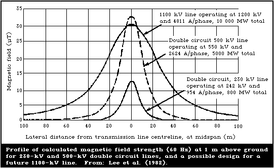 3.2.1.3 Transportation
Several countries are currently designing and testing prototype
vehicles that are suspended and guided by magnetic forces. If
successful, the magnetically-levitated vehicle could offer high-
speed public transportation (roughly 200 - 400 km/h), with greatly
reduced levels of noise and pollution, compared with conventional
modes of transportation.
The technical problems of magnetic levitation are consid-erable
and include the presence of large fringe magnetic fields within the
passenger compartment. In some designs, the field level at the
floor of the passenger compartment may be 50 - 100 mT, and
estimates of the field at the location of a passenger's head range
from 6 to 60 mT (Hassenzahl et al., 1978). The magnetic flux
density within the passenger compartment can be significantly
reduced by several procedures and it may be possible to achieve a
5- to 10-fold reduction in the magnetic field levels to which
passengers are exposed.
3.2.1.4 Security systems
Different security systems have been developed for personnel
identification or for electronic surveillance against theft in
libraries and shops. Such devices operate at frequencies ranging
between 0.1 and 10 kHz. Identification is achieved when a person
passes through the coil carrying an identification tag or articles
bearing a magnetic strip. The maximum magnetic flux generated by
the coil is about 1 mT at the ground.
The maximum magnetic flux for walk-through metal detectors used
at airports is below 0.1 mT, and they have frequencies of operation
below 1 MHz.
3.2.2. Magnetic fields in the work-place
3.2.2.1 Industrial processes
Occupational exposure to magnetic fields comes predominantly
from working near industrial equipment using high currents. Such
devices include various types of welding machine, electroslag
refining, various furnaces, induction heaters, and stirrers.
Details of surveys of magnetic field strengths in industrial
settings are given in Table 6. Surveys on induction heaters used in
industry performed in Canada (Stuchly & Lecuyer, 1985), in Poland
(Aniolczyk, 1981), and in Sweden (Lövsund et al., 1982), show
magnetic flux densities at operator locations ranging from 0.7 µT
to 6 mT, depending on the frequency used and the distance from the
machine. In their study of magnetic fields from industrial
electro-steel and welding equipment, Lövsund et al. (1982) found
that spot welding machines (50 Hz, 15 - 106 kA) and ladle furnaces
(50 Hz, 13 - 15 kA) produced fields up to 10 mT, at distances up to
1 m. In the production of aluminium using a Soderberg cell, the
final reduction process may lead to static field exposures of about
40 mT.
Table 6. Occupational sources of exposure to magnetic fields
----------------------------------------------------------------------
Source Magnetic flux Distance Reference
densities (mT) (m)
----------------------------------------------------------------------
VDTs up - 2.8 x 10⁻⁴ 0.3 Stuchly et al. (1983)
Welding arcs 0.1 - 5.8 0 - 0.8 Lövsund et al. (1982)
(0 - 50 Hz)
Induction heaters 0.9 - 65 0.1 - 1 Lövsund et al. (1982)
(50 - 10 Hz)
50-Hz Ladle 0.2 - 8 0.5 - 1 Lövsund et al. (1982)
furnace
50-Hz Arc up - 1 2 Lövsund et al. (1982)
furnace
10-Hz Induction 0.2 - 0.3 2 Lövsund et al. (1982)
stirrer
50-Hz Electroslag 0.5 - 1.7 0.2 - 0.9 Lövsund et al. (1982)
welding
----------------------------------------------------------------------
Table 6 (contd.)
----------------------------------------------------------------------
Source Magnetic flux Distance Reference
densities (mT) (m)
----------------------------------------------------------------------
Electrolyte 7.6 (mean) operator Marsh et al. (1982)
process position
(0 - 50 Hz)
Isotope 1 - 50 operator Tenforde (1986c)
separation position
(static fields)
----------------------------------------------------------------------
In the course of studies on the health of workers in industries
using electrolytic processes, Marsh et al. (1982) found that the
mean static magnetic field level at operator-accessible locations
was 7.6 mT and the maximum was 14.6 mT. Time-weighted-average field
exposures were calculated to be about 4 and 11.8 mT for the mean
and maximum field levels, respectively.
Vyalov (1974) characterized the average magnetic field levels
to which Soviet workers in permanent magnet production plants were
exposed. He found that the static magnetic field at the level of a
worker's hands was typically 2 - 5 mT. At the level of the chest
and head, the field was generally in the range of 0.3 - 0.5 mT.
3.2.2.2 Energy technologies
High static magnetic field strengths may be encountered around
new and developing technologies used for energy production and
storage, such as magnetohydrodynamic systems, superconducting
magnetic energy storage systems, and thermonuclear fusion
(Tenforde, 1986b).
The thermonuclear fusion process involves the combination of
two light nuclei to form a heavier nucleus with a resultant release
of energy. Various methods can be used to confine an ignited
plasma, including high-intensity magnetic fields. It is now
generally believed that fields as high as 9 - 12 T will be required
for the sustained magnetic confinement of an ignited plasma.
Fringe fields up to 50 mT will exist at locations within the main
reactor building in areas accessible to operations personnel.
Although only a limited number of scientists and maintenance
personnel would normally be expected to enter fields of this
intensity, it is expected that they will do so for brief periods
during normal reactor operation.
Power generation by magnetohydrodynamic (MHD) separation of
ionic charges has been studied as a potential means for increasing
the net power output of a gas- or coal-fired electric power
facility. To a first approximation, a typical MHD generator can be
represented as a magnetic dipole with a large net moment of
approximately 8000 MA x m2 (Hassenzahl et al., 1978). The field
level at a distance of about 50 m from the device would then be
approximately 10 mT and the field level would fall below 0.1 mT
only at distances greater than 250 m.
3.2.2.3 Switching stations and power plants
Typical values for the magnetic flux density at work-places,
near overhead lines, in substations, and in power stations (16,
2/3, 50, 60Hz) range up to 0.05 mT (Krause, 1986).
3.2.2.4 Research facilities
Selected groups of workers in research laboratories may be
exposed to high magnetic field strengths, particularly near bubble
chambers and particle accelerators.
During the last three decades, bubble chambers have played a
major role in the study of high-energy nuclear reactions. The
bubble chamber is contained within a solenoidal magnet operating at
field levels up to approximately 3 T.
At the location where an operator changes the film cassettes,
the field is estimated to be approximately 0.4 - 0.5 T at foot level
and about 0.05 T at the level of the head. The film changing
procedure requires 5 min to complete, and is carried out
approximately three times per day, i.e., once per 8-h work shift
(Tenforde, 1986b).
Linear accelerators and synchrotrons have found applications
in nearly every scientific field, including such areas as high-
energy physics, nuclear chemistry, cancer radiotherapy, and
isotope production for research and medicine. The scale of these
devices ranges from a few metres to several kilometres. Similarly,
the focusing and beam extraction magnets used in various
accelerator designs differ widely in field strengths and in the
magnetic field profile. Although high magnetic fields may be
present near accelerator magnets, personnel are seldom exposed to
these fields, because of exclusion from the high ionizing radiation
zone surrounding the beam line.
3.2.2.5 Video display terminals
The use of computers with screen-based output units or video
display terminals (VDT) grows at an ever increasing rate. VDT
operators have expressed concerns about possible effects from
emissions of low-level radiations. Magnetic fields (frequency 15 -
125 kHz) as high as 0.69 A/m (0.9 µT) have been measured close to
the surface of the screen (Bureau of Radiological Health, 1981)
under worst-case conditions. This result has been confirmed by many
surveys (Roy et al., 1984; Repacholi, 1985a). In a comprehensive
review of measurements and surveys of VDTs by national agencies and
individual experts, it was concluded that there are no radiation
emissions from VDTs that would have any consequences for health
(Repacholi, 1985a). There is no need to perform routine radiation
measurements since, even under worst-case conditions, the emissions
are well below any international or national standards.
3.3. Magnetic Fields in Medical Practice
3.3.1. Diagnosis, magnetic resonance imaging, and metabolic studies
Magnetic resonance (MR) imaging used for diagnostic purposes
involves both static and time-varying magnetic fields. MR imaging
applied to living tissues provides a promising new technique for
medical imaging with high spatial resolutions (Budinger &
Lauterbur, 1984). In this technique, nuclear magnetic moments are
aligned by the application of a static magnetic field (Bo), and
undergo a precessional motion around the field direction with a
Larmor frequency characteristic of each nucleus (section 2.3.3).
When a radiofrequency (RF) field with a matching frequency is
applied transverse to the direction of Bo, a resonant energy
absorption occurs. The return of the magnetic spin state to
equilibrium following resonant energy absorption is characterized
by two relaxation times, T1 and T2. The T1 parameter is called the
spin-lattice relaxation time, and reflects the local temperature
and viscosity in the vicinity of the magnetic nuclei. The T2
parameter is called the "spin-spin" relaxation time, and reflects
the local magnetic field resulting from the nuclear moments of
neighbouring nuclei. Both the T1 and T2 relaxation times provide
information that can be converted into contrast differences in NMR
images of tissue-proton density. The intensity of the radiated
signal reflects the tissue concentration of magnetic nuclei such as
protons, 13C, 23Na, 31P, and 39K. The selective detection of
different magnetic nuclei is possible, because of their different
characteristic resonant frequencies at a given magnetic field
strength.
The decay of a MR signal occurs with a characteristic time
variation that conveys detailed information about the local
environment of the magnetic nuclei. In proton MR images, large
contrast differences can be observed between regions of tissue that
have significantly different water or lipid contents. Various MR
imaging methods have been developed that are able to demonstrate
differences between normal and pathological regions of the same
tissue (Crooks & Kaufman, 1983). Principles and applications of
magnetic resonance techniques in medicine can be found in Mansfield
& Morris (1982), Foster (1984), and Mathur (1984).
In addition to use as an imaging technique, MR spectroscopy
based on 13C and 31P signals can provide unique information on
tissue metabolism. For example, 31P MR spectroscopy has been shown
to give quantitative information on phosphate metabolism in the
heart, liver, kidney, brain, and muscle tissue.
The present generation of MR imaging devices, used in clinical
practice, employ stationary magnetic fields with intensities
ranging from 0.3 T to about 2 T and RF fields with frequencies up
to 100 MHz (the proton resonant frequency in a 2 T field is 85.15
MHz). In addition, weak spatial gradients of the stationary
magnetic field (about 0.001 T/m) are used to define the tissue
location of MR signals. The gradient direction is rapidly switched
from one projection axis to the next in order to reconstruct the
entire image of the specimen. These rapidly switched gradient
fields produce a time-varying magnetic field within the tissue
volume. In the MR imaging devices that are currently in existence,
the maximum time rate of change of the magnetic field is normally
about 1.5 T/second, but may be considerably higher in a few
specialized devices.
The feasibility of using static magnetic fields with strengths
greater than 2T is being explored as a means of increasing the
signal-to-noise ratio in MR images. In addition, the use of higher
fields could significantly reduce the time required to obtain
chemical shift images, which provide high-resolution information on
the spatial distribution of 31P nuclei and protons associated with
tissue water and fat.
3.3.2. Therapy
Patients suffering from bone fractures that do not heal well or
unite have been treated with pulsed magnetic fields (Bassett et
al., 1974, 1977, 1982; Mitbreit & Manyachin, 1984). Studies are
also being conducted on the use of pulsed magnetic fields to
enhance wound healing and tissue regeneration.
Various devices generating magnetic field pulses are used for
bone growth stimulation. A typical example is the device that
generates an average magnetic flux density of about 0.3 mT, a peak
strength of about 2.5 mT, and induces peak electric field strengths
in the bone in the range of 0.075 - 0.175 V/m (Bassett et al.,
1974). Two different pulse patterns are used: a quasi-rectangular
pulse of 250 - 400 µs duration with a secondary pulse of opposite
polarity of 20 µs width, and a repetition rate of 40 - 77 Hz; and a
train of pulses with a duration of 2.5 ms and a repetition rate of
5 - 20 Hz (Fig. 3). Near the surface of the exposed limb, the
device produces a peak magnetic flux density of the order of 1.0 mT
causing peak ionic current densities of about 10 to 100 mA/m2 (1 to
10 µA/cm2) in tissue. These ionic currents perturb cell function,
even though most of the current flows around the cell in the
extracellular space (Pilla, 1979; Beltrame et al., 1980; Pilla et
al., 1983). Applications of magnetic field devices in medicine are
rapidly expanding. Further information can be obtained in the
monograph edited by Bistolfi (1983). Magnetic fields are being
widely used in the USSR for various therapeutic applications
(Bogolyubov, 1981).
3.2.1.3 Transportation
Several countries are currently designing and testing prototype
vehicles that are suspended and guided by magnetic forces. If
successful, the magnetically-levitated vehicle could offer high-
speed public transportation (roughly 200 - 400 km/h), with greatly
reduced levels of noise and pollution, compared with conventional
modes of transportation.
The technical problems of magnetic levitation are consid-erable
and include the presence of large fringe magnetic fields within the
passenger compartment. In some designs, the field level at the
floor of the passenger compartment may be 50 - 100 mT, and
estimates of the field at the location of a passenger's head range
from 6 to 60 mT (Hassenzahl et al., 1978). The magnetic flux
density within the passenger compartment can be significantly
reduced by several procedures and it may be possible to achieve a
5- to 10-fold reduction in the magnetic field levels to which
passengers are exposed.
3.2.1.4 Security systems
Different security systems have been developed for personnel
identification or for electronic surveillance against theft in
libraries and shops. Such devices operate at frequencies ranging
between 0.1 and 10 kHz. Identification is achieved when a person
passes through the coil carrying an identification tag or articles
bearing a magnetic strip. The maximum magnetic flux generated by
the coil is about 1 mT at the ground.
The maximum magnetic flux for walk-through metal detectors used
at airports is below 0.1 mT, and they have frequencies of operation
below 1 MHz.
3.2.2. Magnetic fields in the work-place
3.2.2.1 Industrial processes
Occupational exposure to magnetic fields comes predominantly
from working near industrial equipment using high currents. Such
devices include various types of welding machine, electroslag
refining, various furnaces, induction heaters, and stirrers.
Details of surveys of magnetic field strengths in industrial
settings are given in Table 6. Surveys on induction heaters used in
industry performed in Canada (Stuchly & Lecuyer, 1985), in Poland
(Aniolczyk, 1981), and in Sweden (Lövsund et al., 1982), show
magnetic flux densities at operator locations ranging from 0.7 µT
to 6 mT, depending on the frequency used and the distance from the
machine. In their study of magnetic fields from industrial
electro-steel and welding equipment, Lövsund et al. (1982) found
that spot welding machines (50 Hz, 15 - 106 kA) and ladle furnaces
(50 Hz, 13 - 15 kA) produced fields up to 10 mT, at distances up to
1 m. In the production of aluminium using a Soderberg cell, the
final reduction process may lead to static field exposures of about
40 mT.
Table 6. Occupational sources of exposure to magnetic fields
----------------------------------------------------------------------
Source Magnetic flux Distance Reference
densities (mT) (m)
----------------------------------------------------------------------
VDTs up - 2.8 x 10⁻⁴ 0.3 Stuchly et al. (1983)
Welding arcs 0.1 - 5.8 0 - 0.8 Lövsund et al. (1982)
(0 - 50 Hz)
Induction heaters 0.9 - 65 0.1 - 1 Lövsund et al. (1982)
(50 - 10 Hz)
50-Hz Ladle 0.2 - 8 0.5 - 1 Lövsund et al. (1982)
furnace
50-Hz Arc up - 1 2 Lövsund et al. (1982)
furnace
10-Hz Induction 0.2 - 0.3 2 Lövsund et al. (1982)
stirrer
50-Hz Electroslag 0.5 - 1.7 0.2 - 0.9 Lövsund et al. (1982)
welding
----------------------------------------------------------------------
Table 6 (contd.)
----------------------------------------------------------------------
Source Magnetic flux Distance Reference
densities (mT) (m)
----------------------------------------------------------------------
Electrolyte 7.6 (mean) operator Marsh et al. (1982)
process position
(0 - 50 Hz)
Isotope 1 - 50 operator Tenforde (1986c)
separation position
(static fields)
----------------------------------------------------------------------
In the course of studies on the health of workers in industries
using electrolytic processes, Marsh et al. (1982) found that the
mean static magnetic field level at operator-accessible locations
was 7.6 mT and the maximum was 14.6 mT. Time-weighted-average field
exposures were calculated to be about 4 and 11.8 mT for the mean
and maximum field levels, respectively.
Vyalov (1974) characterized the average magnetic field levels
to which Soviet workers in permanent magnet production plants were
exposed. He found that the static magnetic field at the level of a
worker's hands was typically 2 - 5 mT. At the level of the chest
and head, the field was generally in the range of 0.3 - 0.5 mT.
3.2.2.2 Energy technologies
High static magnetic field strengths may be encountered around
new and developing technologies used for energy production and
storage, such as magnetohydrodynamic systems, superconducting
magnetic energy storage systems, and thermonuclear fusion
(Tenforde, 1986b).
The thermonuclear fusion process involves the combination of
two light nuclei to form a heavier nucleus with a resultant release
of energy. Various methods can be used to confine an ignited
plasma, including high-intensity magnetic fields. It is now
generally believed that fields as high as 9 - 12 T will be required
for the sustained magnetic confinement of an ignited plasma.
Fringe fields up to 50 mT will exist at locations within the main
reactor building in areas accessible to operations personnel.
Although only a limited number of scientists and maintenance
personnel would normally be expected to enter fields of this
intensity, it is expected that they will do so for brief periods
during normal reactor operation.
Power generation by magnetohydrodynamic (MHD) separation of
ionic charges has been studied as a potential means for increasing
the net power output of a gas- or coal-fired electric power
facility. To a first approximation, a typical MHD generator can be
represented as a magnetic dipole with a large net moment of
approximately 8000 MA x m2 (Hassenzahl et al., 1978). The field
level at a distance of about 50 m from the device would then be
approximately 10 mT and the field level would fall below 0.1 mT
only at distances greater than 250 m.
3.2.2.3 Switching stations and power plants
Typical values for the magnetic flux density at work-places,
near overhead lines, in substations, and in power stations (16,
2/3, 50, 60Hz) range up to 0.05 mT (Krause, 1986).
3.2.2.4 Research facilities
Selected groups of workers in research laboratories may be
exposed to high magnetic field strengths, particularly near bubble
chambers and particle accelerators.
During the last three decades, bubble chambers have played a
major role in the study of high-energy nuclear reactions. The
bubble chamber is contained within a solenoidal magnet operating at
field levels up to approximately 3 T.
At the location where an operator changes the film cassettes,
the field is estimated to be approximately 0.4 - 0.5 T at foot level
and about 0.05 T at the level of the head. The film changing
procedure requires 5 min to complete, and is carried out
approximately three times per day, i.e., once per 8-h work shift
(Tenforde, 1986b).
Linear accelerators and synchrotrons have found applications
in nearly every scientific field, including such areas as high-
energy physics, nuclear chemistry, cancer radiotherapy, and
isotope production for research and medicine. The scale of these
devices ranges from a few metres to several kilometres. Similarly,
the focusing and beam extraction magnets used in various
accelerator designs differ widely in field strengths and in the
magnetic field profile. Although high magnetic fields may be
present near accelerator magnets, personnel are seldom exposed to
these fields, because of exclusion from the high ionizing radiation
zone surrounding the beam line.
3.2.2.5 Video display terminals
The use of computers with screen-based output units or video
display terminals (VDT) grows at an ever increasing rate. VDT
operators have expressed concerns about possible effects from
emissions of low-level radiations. Magnetic fields (frequency 15 -
125 kHz) as high as 0.69 A/m (0.9 µT) have been measured close to
the surface of the screen (Bureau of Radiological Health, 1981)
under worst-case conditions. This result has been confirmed by many
surveys (Roy et al., 1984; Repacholi, 1985a). In a comprehensive
review of measurements and surveys of VDTs by national agencies and
individual experts, it was concluded that there are no radiation
emissions from VDTs that would have any consequences for health
(Repacholi, 1985a). There is no need to perform routine radiation
measurements since, even under worst-case conditions, the emissions
are well below any international or national standards.
3.3. Magnetic Fields in Medical Practice
3.3.1. Diagnosis, magnetic resonance imaging, and metabolic studies
Magnetic resonance (MR) imaging used for diagnostic purposes
involves both static and time-varying magnetic fields. MR imaging
applied to living tissues provides a promising new technique for
medical imaging with high spatial resolutions (Budinger &
Lauterbur, 1984). In this technique, nuclear magnetic moments are
aligned by the application of a static magnetic field (Bo), and
undergo a precessional motion around the field direction with a
Larmor frequency characteristic of each nucleus (section 2.3.3).
When a radiofrequency (RF) field with a matching frequency is
applied transverse to the direction of Bo, a resonant energy
absorption occurs. The return of the magnetic spin state to
equilibrium following resonant energy absorption is characterized
by two relaxation times, T1 and T2. The T1 parameter is called the
spin-lattice relaxation time, and reflects the local temperature
and viscosity in the vicinity of the magnetic nuclei. The T2
parameter is called the "spin-spin" relaxation time, and reflects
the local magnetic field resulting from the nuclear moments of
neighbouring nuclei. Both the T1 and T2 relaxation times provide
information that can be converted into contrast differences in NMR
images of tissue-proton density. The intensity of the radiated
signal reflects the tissue concentration of magnetic nuclei such as
protons, 13C, 23Na, 31P, and 39K. The selective detection of
different magnetic nuclei is possible, because of their different
characteristic resonant frequencies at a given magnetic field
strength.
The decay of a MR signal occurs with a characteristic time
variation that conveys detailed information about the local
environment of the magnetic nuclei. In proton MR images, large
contrast differences can be observed between regions of tissue that
have significantly different water or lipid contents. Various MR
imaging methods have been developed that are able to demonstrate
differences between normal and pathological regions of the same
tissue (Crooks & Kaufman, 1983). Principles and applications of
magnetic resonance techniques in medicine can be found in Mansfield
& Morris (1982), Foster (1984), and Mathur (1984).
In addition to use as an imaging technique, MR spectroscopy
based on 13C and 31P signals can provide unique information on
tissue metabolism. For example, 31P MR spectroscopy has been shown
to give quantitative information on phosphate metabolism in the
heart, liver, kidney, brain, and muscle tissue.
The present generation of MR imaging devices, used in clinical
practice, employ stationary magnetic fields with intensities
ranging from 0.3 T to about 2 T and RF fields with frequencies up
to 100 MHz (the proton resonant frequency in a 2 T field is 85.15
MHz). In addition, weak spatial gradients of the stationary
magnetic field (about 0.001 T/m) are used to define the tissue
location of MR signals. The gradient direction is rapidly switched
from one projection axis to the next in order to reconstruct the
entire image of the specimen. These rapidly switched gradient
fields produce a time-varying magnetic field within the tissue
volume. In the MR imaging devices that are currently in existence,
the maximum time rate of change of the magnetic field is normally
about 1.5 T/second, but may be considerably higher in a few
specialized devices.
The feasibility of using static magnetic fields with strengths
greater than 2T is being explored as a means of increasing the
signal-to-noise ratio in MR images. In addition, the use of higher
fields could significantly reduce the time required to obtain
chemical shift images, which provide high-resolution information on
the spatial distribution of 31P nuclei and protons associated with
tissue water and fat.
3.3.2. Therapy
Patients suffering from bone fractures that do not heal well or
unite have been treated with pulsed magnetic fields (Bassett et
al., 1974, 1977, 1982; Mitbreit & Manyachin, 1984). Studies are
also being conducted on the use of pulsed magnetic fields to
enhance wound healing and tissue regeneration.
Various devices generating magnetic field pulses are used for
bone growth stimulation. A typical example is the device that
generates an average magnetic flux density of about 0.3 mT, a peak
strength of about 2.5 mT, and induces peak electric field strengths
in the bone in the range of 0.075 - 0.175 V/m (Bassett et al.,
1974). Two different pulse patterns are used: a quasi-rectangular
pulse of 250 - 400 µs duration with a secondary pulse of opposite
polarity of 20 µs width, and a repetition rate of 40 - 77 Hz; and a
train of pulses with a duration of 2.5 ms and a repetition rate of
5 - 20 Hz (Fig. 3). Near the surface of the exposed limb, the
device produces a peak magnetic flux density of the order of 1.0 mT
causing peak ionic current densities of about 10 to 100 mA/m2 (1 to
10 µA/cm2) in tissue. These ionic currents perturb cell function,
even though most of the current flows around the cell in the
extracellular space (Pilla, 1979; Beltrame et al., 1980; Pilla et
al., 1983). Applications of magnetic field devices in medicine are
rapidly expanding. Further information can be obtained in the
monograph edited by Bistolfi (1983). Magnetic fields are being
widely used in the USSR for various therapeutic applications
(Bogolyubov, 1981).
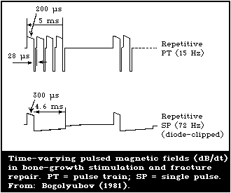 4. MECHANISMS OF INTERACTION
A broad spectrum of interaction mechanisms can occur between
magnetic fields and living tissue. At the level of macromolecules
and larger structures, interactions of stationary magnetic fields
with biological systems can be characterized as electrodynamic or
magnetomechanical in nature. Electrodynamic effects originate
through the interaction of magnetic fields with electrolyte flows,
leading to the induction of electrical potentials and currents.
Magnetomechanical phenomena include orientational effects on
macromolecular assemblies in homogeneous fields, and the
translation of paramagnetic and ferromagnetic molecular species in
strong gradient fields. Magnetic fields that are time-varying also
interact with living tissues at the macroscopic and microscopic
levels to produce circulating currents via the mechanism of
magnetic induction. The theory behind each of these interaction
mechanisms will be described in this section.
At the atomic and subatomic levels, several types of magnetic
field interactions have been shown to occur in biological systems
(Cope, 1971, 1973, 1978, 1981). Two such interactions are the
nuclear magnetic resonance in living tissues described earlier and
the effects on electronic spin states and their relevance to
certain classes of electron transfer reactions described in this
section.
Other interaction mechanisms that are being studied at the
present time are discussed at the end of this section. Recent
reviews of the theoretical bases for magnetic field interactions
include those of Bernhardt (1979, 1986), Schulten (1982, 1986),
Pirusyan & Kuznetsov (1983), Abashin & Yevtushenko (1984), Swicord
(1985); Tenforde (1985a,c, 1986a,d), Kaune (1985), Frankel (1986),
and Tenforde & Budinger (1986).
4.1. Static Magnetic Fields
4.1.1. Electrodynamic and magnetohydrodynamic interactions
Steady flows of ionic currents interact with applied stationary
magnetic fields via the well known Lorentz force law (equation 3):
F = q (v x B) (3)
where F is the net force exerted on a charge q moving with velocity
v, and B is the magnetic flux density. The term v x B represents a
vector cross-product. In the case of electrolytes flowing through
channels (e.g., blood vessels), the interaction of an applied
magnetic field with ionic charge carriers under steady-state
conditions will result in a local force on the charge carriers of
magnitude q v B sin THETA where THETA is the angle between the
direction of charge motion and the magnetic field. This force will
be perpendicular to both the magnetic field and the direction of
current flow, i.e., the induced field, Ei, is transverse to both
v and B. This phenomenon, which is the basis of the Hall effect in
solid state materials, is also relevant to biological processes that
involve electrolyte flow.
An interesting example of the role of magnetically-induced
electrical potentials in a biological system is the geo-magnetic
direction-finding mechanism used by elasmobranch fish, including
the shark, skate, and ray (Kalmijn, 1974, 1978, 1981, 1984; Ilinsky
& Brown, 1985). The heads of these animals contain long jelly-
filled canals known as the ampullae of Lorenzini, which have a high
electrical conductivity similar to that of seawater. As the fish
swims through the earth's magnetic field, a small voltage gradient
is induced in the canals, which is detected by the sensory
epithelia lining the terminal ampullary region. The induced
electric field, which can be detected at levels as low as 0.5 µV/m
(Kalmijn, 1982), has a distinct polarity that is dependent on the
relative orientation of the geomagnetic field direction of swimming.
In this way, the marine elasmobranchs use the -(v x B) fields
induced in their ampullary canals as a directional compass.
A second example of induced electric potentials is provided by
blood flow in the presence of an applied static magnetic field.
For the specific case of a cylindrical vessel with a diameter (d)
and the local electric field strength (Ei), the magnitude of the
induced potential PSI, is given by equation 4:
PSI = |Ei|d = |v||B|d sin THETA (4)
The existence of magnetically-induced blood flow potentials in
the central circulatory systems of several species of mammals has
been demonstrated experimentally. These induced potentials can be
conveniently studied from electrocardiogram (ECG) records obtained
with surface electrodes. The ECG signal in the T-wave region shows
a substantial augmentation in the presence of magnetic fields and
this phenomenon is completely and immediately reversible on
termination of the exposure. Based on its temporal sequence in the
ECG record, the increased amplitude of the T-wave in magnetic
fields has been attributed to the superposition of an induced
potential associated with pulsatile blood flow into the aortic
vessel. This effect is illustrated in Fig. 4 and discussed in more
detail in section 5. The occurrence of a change in the ECG is an
excellent example of a physical effect of an applied magnetic field
that does not result from a biological response to the field.
For a man with a peak blood flow rate of 0.63 m/s and an aortic
diameter of 0.025 m, the predicted maximum value of the aortic flow
potential is 16 mV per tesla (Mansfield & Morris, 1982). The
actual potential across the cardiac muscle fibres would be much
smaller, so that the threshold change in cardiac potential required
to initiate depolarization of cardiac muscle may not be reached,
even in magnetic fields of a few tesla. However, the induced
potential differences can be significant in cases where the
excitation stimulation or conduction of excitation is impaired.
This is one of the reasons why, in recommendations for the safe
medical use of magnetic resonance equipment where a field of more
than 2 T is used, monitoring of cardiac and circulatory function of
the patient is recommended (Bernhardt & Kossel, 1984, 1985).
4. MECHANISMS OF INTERACTION
A broad spectrum of interaction mechanisms can occur between
magnetic fields and living tissue. At the level of macromolecules
and larger structures, interactions of stationary magnetic fields
with biological systems can be characterized as electrodynamic or
magnetomechanical in nature. Electrodynamic effects originate
through the interaction of magnetic fields with electrolyte flows,
leading to the induction of electrical potentials and currents.
Magnetomechanical phenomena include orientational effects on
macromolecular assemblies in homogeneous fields, and the
translation of paramagnetic and ferromagnetic molecular species in
strong gradient fields. Magnetic fields that are time-varying also
interact with living tissues at the macroscopic and microscopic
levels to produce circulating currents via the mechanism of
magnetic induction. The theory behind each of these interaction
mechanisms will be described in this section.
At the atomic and subatomic levels, several types of magnetic
field interactions have been shown to occur in biological systems
(Cope, 1971, 1973, 1978, 1981). Two such interactions are the
nuclear magnetic resonance in living tissues described earlier and
the effects on electronic spin states and their relevance to
certain classes of electron transfer reactions described in this
section.
Other interaction mechanisms that are being studied at the
present time are discussed at the end of this section. Recent
reviews of the theoretical bases for magnetic field interactions
include those of Bernhardt (1979, 1986), Schulten (1982, 1986),
Pirusyan & Kuznetsov (1983), Abashin & Yevtushenko (1984), Swicord
(1985); Tenforde (1985a,c, 1986a,d), Kaune (1985), Frankel (1986),
and Tenforde & Budinger (1986).
4.1. Static Magnetic Fields
4.1.1. Electrodynamic and magnetohydrodynamic interactions
Steady flows of ionic currents interact with applied stationary
magnetic fields via the well known Lorentz force law (equation 3):
F = q (v x B) (3)
where F is the net force exerted on a charge q moving with velocity
v, and B is the magnetic flux density. The term v x B represents a
vector cross-product. In the case of electrolytes flowing through
channels (e.g., blood vessels), the interaction of an applied
magnetic field with ionic charge carriers under steady-state
conditions will result in a local force on the charge carriers of
magnitude q v B sin THETA where THETA is the angle between the
direction of charge motion and the magnetic field. This force will
be perpendicular to both the magnetic field and the direction of
current flow, i.e., the induced field, Ei, is transverse to both
v and B. This phenomenon, which is the basis of the Hall effect in
solid state materials, is also relevant to biological processes that
involve electrolyte flow.
An interesting example of the role of magnetically-induced
electrical potentials in a biological system is the geo-magnetic
direction-finding mechanism used by elasmobranch fish, including
the shark, skate, and ray (Kalmijn, 1974, 1978, 1981, 1984; Ilinsky
& Brown, 1985). The heads of these animals contain long jelly-
filled canals known as the ampullae of Lorenzini, which have a high
electrical conductivity similar to that of seawater. As the fish
swims through the earth's magnetic field, a small voltage gradient
is induced in the canals, which is detected by the sensory
epithelia lining the terminal ampullary region. The induced
electric field, which can be detected at levels as low as 0.5 µV/m
(Kalmijn, 1982), has a distinct polarity that is dependent on the
relative orientation of the geomagnetic field direction of swimming.
In this way, the marine elasmobranchs use the -(v x B) fields
induced in their ampullary canals as a directional compass.
A second example of induced electric potentials is provided by
blood flow in the presence of an applied static magnetic field.
For the specific case of a cylindrical vessel with a diameter (d)
and the local electric field strength (Ei), the magnitude of the
induced potential PSI, is given by equation 4:
PSI = |Ei|d = |v||B|d sin THETA (4)
The existence of magnetically-induced blood flow potentials in
the central circulatory systems of several species of mammals has
been demonstrated experimentally. These induced potentials can be
conveniently studied from electrocardiogram (ECG) records obtained
with surface electrodes. The ECG signal in the T-wave region shows
a substantial augmentation in the presence of magnetic fields and
this phenomenon is completely and immediately reversible on
termination of the exposure. Based on its temporal sequence in the
ECG record, the increased amplitude of the T-wave in magnetic
fields has been attributed to the superposition of an induced
potential associated with pulsatile blood flow into the aortic
vessel. This effect is illustrated in Fig. 4 and discussed in more
detail in section 5. The occurrence of a change in the ECG is an
excellent example of a physical effect of an applied magnetic field
that does not result from a biological response to the field.
For a man with a peak blood flow rate of 0.63 m/s and an aortic
diameter of 0.025 m, the predicted maximum value of the aortic flow
potential is 16 mV per tesla (Mansfield & Morris, 1982). The
actual potential across the cardiac muscle fibres would be much
smaller, so that the threshold change in cardiac potential required
to initiate depolarization of cardiac muscle may not be reached,
even in magnetic fields of a few tesla. However, the induced
potential differences can be significant in cases where the
excitation stimulation or conduction of excitation is impaired.
This is one of the reasons why, in recommendations for the safe
medical use of magnetic resonance equipment where a field of more
than 2 T is used, monitoring of cardiac and circulatory function of
the patient is recommended (Bernhardt & Kossel, 1984, 1985).
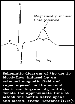 Potential differences may also be induced by moving cross
sections in a magnetic field, e.g. by cardiac contractions. In
theory (Bernhardt & Kossel, 1984), a field strength of 0.1 V/m or a
current density of about 10 - 20 mA/m2 per tesla is induced in
cardiac muscle. A large current density in the vicinity of the
heart may cause ventricular fibrillation. However, the threshold
magnetic field strengths for the induction of effects on cardiac
function, including alteration of excitation or impulse conduction,
are not known.
Another biological process involving ionic flows that are
subject to electrodynamic interaction with an applied magnetic
field is the conduction of electrical impulses in nerve tissue.
Wikswo & Barach (1980) have calculated that a magnetic field
strength of 24 T could produce a deflecting force on nerve ionic
currents equal to one tenth of the force that they experience from
interaction with the electric field of the nerve membrane. A
theoretical model suggests that magnetic fields with flux densities
of 2 T or less should not produce any measurable change in the
conduction velocity of nerve impulses. This conclusion is supported
by experimental data (section 5).
Theoretical analyses of magnetic field interactions with nerve
ionic currents have also been made by Valentinuzzi (1965) and
Liboff (1980). Liboff has raised the interesting question of
whether time variations in the magnetic flux linkage with ion
current loops along the nerve membrane could lead to significant
induced potentials. Due to the rotational symmetry of the nerve
axon, it is expected that these induced electrical fields would
cancel. However, for the unlikely condition of highly asymmetric
current loops, Liboff (1980) suggests that applied fields of less
than 1 T could theoretically introduce significant perturbations in
the membrane current flows during impulse conduction. At present,
there are not sufficient data to test this hypothesis.
Theoretically, intracellular ionic fluxes are also susceptible
to magnetic field interaction, but there is little experimental
information relating to this possibility (Czerski, 1986).
4.1.2. Magnetomechanical effects
4.1.2.1 Orientation of diamagnetically anisotropic macromolecules
A large number of diamagnetic biological macromolecules exhibit
orientation in strong magnetic fields. In general, these
macromolecules have a rod-like shape, and magneto-orientation
occurs as a result of an anisotropy in the magnetic susceptibility
tensor (x) along the different axes of rotational symmetry. The
magnetic moment per unit volume (M) of these molecules in a field
with intensity H is equal to xH. The theoretical calculation of
the interaction energy per unit volume has been discussed by
Tenforde (1985a) and Frankel (1986). The rod-like molecules will
rotate to achieve a minimum energy in the applied magnetic field.
For individual macromolecules, the magnetic interaction energy
predicted theoretically will be small compared to the thermal
interaction energy kT, unless enormous field strengths are used.
This fact has been demonstrated for DNA solutions in which the
extent of magneto-orientation has been studied from measurements of
magnetically-induced bire-fringence (the Cotton-Mouton effect).
Measurements on calf thymus DNA (Maret et al., 1975; Maret &
Dransfeld, 1977), resulted in a degree of orientation of only 1% in
an applied field of 13 T.
Despite the weak interaction of individual macromolecules with
intense magnetic fields, there are several examples of
macromolecular assemblies that exhibit orientation in fields of 1 T
or less. This phenomenon results from a summation of the
diamagnetic anisotropies of the individual molecules within the
assembly, thereby giving rise to a large effective anisotropy and
magnetic interaction energy for the entire molecular aggregate.
Examples of biological systems that exhibit orientation in fields
of 1 T or less are retinal rod outer segments (Chalazonitis et al.,
1970; Hong et al., 1971; Vilenchik, 1982), photosynthetic systems
such as chloroplast grana, photosynthetic bacteria, and Chlorella
cells (Geacintov et al., 1971, 1972; Becker et al., 1973, 1978a,b;
Breton, 1974), purple membranes of Halobacteria (Neugebauer et al.,
1977), muscle fibres (Arnold et al., 1958), and "sickled"
erythrocytes (Murayama, 1965). A more detailed discussion can be
found in Maret & Dransfield (1985).
Several of the physical principles underlying magneto-
orientation phenomena have been experimentally demonstrated for
retinal rod outer segments. The first observation that isolated
rod outer segments, which consist of pigmented disc membranes
stacked in a regular array, will orient in a 1 T stationary
magnetic field was made in 1970 (Chalazonitis et al., 1970). The
oriented segments are aligned with the disc membranes perpendicular
to the applied field direction, which indicates that magneto-
orientation results from the large summed diamagnetic anisotropy of
the rhodopsin photopigments, as opposed to the lamellar membrane
phospholipids (Hong, 1980; Becker et al., 1978b). An estimate of
the summed anisotropy for the rod outer segments can be obtained by
observing the kinetics of the magneto-orientation process. The time
for rods to rotate by 90° is predicted to be approximately 4
seconds in a 1.0 T field (Hong et al., 1971; Hong, 1977, 1980), and
this value agrees well with experimental observations on the
kinetics of rod orientation (Chagneux & Chalazonitis, 1972;
Chagneux et al., 1977). It should be noted that the slow
orientational response of rod outer segments to an applied magnetic
field makes this mechanism an unlikely basis for the
magnetophosphene phenomenon that is observed in time-varying
fields.
4.1.2.2 Orientation of organisms with permanent magnetic moments
An interesting specimen for the biophysical study of magnetic
field interactions was provided by Blakemore's accidental discovery
of magnetotactic bacteria (Blakemore, 1975). Approximately 2% of
the dry mass of these aquatic organisms is iron, which has been
shown by Mossbauer spectroscopy to be predominantly in the form of
magnetite (Fe3O4) (Frankel et al., 1979). The magnetite inclusions
are arranged as chains of approximately 20 - 30 single domain
crystals. The orientation of the net magnetic moment is such that
magnetotactic bacteria in the northern hemisphere migrate towards
the north pole of the geomagnetic field, whereas strains of these
bacteria that grow in the southern hemisphere move towards the
south magnetic pole (Blakemore et al., 1980; Rosenblatt et al.,
1982a,b). Magnetotactic bacteria that have been found at the
geomagnetic equator are nearly equal mixtures of south-seeking and
north-seeking organisms (Frankel et al., 1981). Because of the
polarities of their magnetic moments, the magnetotactic bacteria in
both the northern and southern hemispheres migrate downwards in
response to the vertical component of the geomagnetic field. It
has been proposed that this downward directed motion, which carries
the bacteria into the bottom sediments of their aquatic environment,
is essential for the survival of these microaerophilic organisms
(Blakemore, 1975; Frankel et al., 1979). This phenomenon is an
interesting example of an interaction between a physical response
to a magnetic field and biological environmental adaptation and
selection processes.
4.1.2.3 Translation of substances in a magnetic field gradient
A material with a net magnetic moment will experience a force
in a magnetic field gradient (spatially non-uniform magnetic
field). As a result of this force, paramagnetic and ferromagnetic
materials will migrate along the direction of the magnetic field
gradient.
One of the interesting applications of the magnetomechanical
force exerted by a magnetic field gradient is the differential
separation of erythrocytes from whole blood (Melville et al., 1975;
Paul et al., 1978). In this procedure, deoxygenated erythrocytes,
in which the haemoglobin is paramagnetic, are attracted to a wire
mesh with a strong gradient field and thereby separated from other
classes of blood cells. Magneto-mechanical forces are also applied
in: surgical traumatology to fix skeleton elements in specific
position (Yarovitsky, 1986); in designs of various intestinal and
oesophageal valves; and for the accumulation of drugs (in compounds
with ferromagnetics) in specific parts of the human body. In
ophthalmology, strong constant magnets are applied to extract
foreign (ferromagnetic) objects.
An important safety consideration is the displacement of
metallic inclusions or implants in human beings exposed to strong
magnetic field gradients, as this could pose a health risk (New et
al., 1983).
4.1.3. Effects on electronic spin states
A number of organic reaction processes that involve electron
transfer via radical pair intermediates are highly sensitive to
magnetic field interactions. A well-studied example that is
biologically relevant is the photo-induced charge transfer reaction
that occurs in bacterial photosynthesis (Blankenship et al., 1977;
Werner et al., 1978; Haberhorn & Michel-Beyerle, 1979; Michel-
Beyerle et al., 1979; Hoff, 1981; Ogrodnik et al., 1982). Within
10 picoseconds (ps) following excitation of bacteriochlorophyll
(BChl) to its first excited singlet state, a radical pair
intermediate state is formed that consists of a (BChl)+2 cationic
dimer and a bacteriopheophytin (BPh)- anion. Within 200 ps,
electron transfer occurs to the ultimate acceptor, an ubiquinone-
iron complex. However, if the acceptor molecule is chemically
reduced, the lifetime of the radical pair intermediate state
increases to approximately 10 nanoseconds (ns). With an extended
lifetime, hyperfine interactions between the nuclear and electron
spin magnetic moments lead to an interconversion of the radical
pairs between the singlet and triplet states. Under this condition,
the intermediate state decays directly back to the singlet ground
state, or decays via a metastable triplet state. Because of the
weakness of the hyperfine interaction, the triplet states are
nearly degenerate and the electron spins of the radical pair
intermediate can move with nearly equal probabilities between the
singlet So and the triplet To and T±1 states. However, in the
presence of an applied magnetic field that exceeds approximately 10
mT, the resulting Zeeman interaction with the radical electron
spins will lift the degeneracy of the triplet state and effectively
block the T±1 triplet channels. Theoretically, the yield of
triplet product should be reduced by two thirds in the presence of
the external field, and this has been confirmed experimentally by
laser pulse excitation and optical absorption measurements (Michel-
Beyerle et al., 1979).
In considering the biological implication of these studies, it
should be kept in mind that the ultimate electron acceptor
molecules have been altered by chemical reduction and such
conditions do not normally occur in nature. However, the
possibility cannot be excluded that similar phenomena may occur in
other radical-mediated biological processes under normal
conditions. It has been proposed, for example, by Schulten et al.
(1978), that an anisotropic Zeeman interaction with a radical
mediated reaction system could provide a basis for geomagnetic
direction finding.
Magnetic field effects on organic chemical reactions in which
the splitting and subsequent recombination of a non-excited singlet
molecule involves a radical pair as a short-lived intermediate
stage have also been well documented (Molin et al., 1979;
McLauchlan, 1981). As described above, the effect of the magnetic
field is on the singlet-triplet transition rate of the radical
pair, thus affecting the relative proportion of recombinant and
escape products, by up to 30% in some cases. The magnitude of the
response depends on the difference in the magnetic properties of
the two radical intermediates, and will be particularly enhanced in
reactions involving transition metals such as iron (Molin et al.,
1979). These effects also increase with the lifetime of the
radical pair. This is typically 100 ps - 100 ns in solution, but
is longer when the reacting molecule is held in a micellar "cage"
or bound to an enzyme.
A number of enzyme reactions involving radical intermediates
have been identified (Saunders & Cass, 1983), though the evidence
is tenuous because they are generated and react at the enzyme
active site and their presence can only be inferred by indirect
methods. Enzymes, the action of which may involve radical
intermediates, are:
(a) Cytochrome P-450: A class of haem-containing enzyme
involved in drug metabolism and steroid hydroxylation;
(b) Lipoxygenase: A non-haem iron enzyme that is a key
enzyme in prostaglandin and thromboxane synthesis; and
(c) Cyclo-oxygenase: The enzyme involved in converting
arachadonic acid to prostaglandins.
These enzymes all contain iron and use oxygen (O2) as one of the
substrates. They can be expected to be sensitive to magnetic
fields, if the radical recombination is rate determining, i.e., if
the radical is relatively long-lived.
4.2. Time-Varying Magnetic Fields
In accordance with Faraday's law, magnetic fields that vary in
time will induce potentials and circulating currents in biological
systems.
pi r2 dB sigma r dB
J = E sigma = ------- x -- x sigma = ------- -- (5)
2 pi r dt 2 dt
where J = current density (A/m2)
E = induced potential (V/m)
r = radius of the inductive loop (m)
sigma = tissue conductivity (S/m)
dB = rate of change of magnetic flux density
dt
For sinusoidal fields of frequency f, equation (5) reduces to:
J = pi r f sigma Bo,
where Bo is the magnetic field amplitude
Thus, the magnitude of the induced electric fields and current
densities is proportional to the radius of the loop, the tissue
conductivity, and the rate of change of magnetic flux density.
The dependence of the induced field and current on the radius
of the loop through which magnetic flux linkage occurs is an
important consideration for biological systems. Time-varying
fields of modest strength may induce significant circulating
currents at the macroscopic level, but substantially smaller
currents at the cellular level.
An important factor to be considered in the response of
biological systems to a time-varying magnetic field is the
waveform. Many different types of magnetic field waveform are used
in practice, including sinusoidal, square-wave, saw tooth, and
pulsed fields. For these fields, the two parameters of key
importance are the rise and decay times of the signal, which
determine the maximum time rates of change of the field, (dB/dt),
and hence the maximum instantaneous current densities induced in
tissues. These also depend on tissue conductivity, which is
frequency dependent and differs between tissues.
Luben et al. (1982) and Cain et al. (1984) demonstrated in
vitro that pulsed magnetic fields, generated in pulse trains (72
Hz) or recurrent bursts (15 Hz), blocked the response of mouse
osteoblasts to parathyroid hormone. The effects seemed to be
mediated at the cell membrane by blocking receptor-adenylate
cyclase coupling in the membrane (Cain et al., 1985). The
adenylate cyclase and cyclic AMP systems are part of the hormone
response amplification system. These effects were associated with
current densities of 10 - 100 mA/m2 and electric field strengths of
0.1 - 1 V/m in extracellular fluids. Effects at the cell membrane
receptor level seem to be involved in the effects of 450 MHz fields
sinusoidally modulated at ELF frequencies on T-lymphocyte cytotoxic
functions (Lyle et al., 1983).
Numerous effects resulting ELF electric fields in cells and
tissues, induced by pulsed magnetic fields, have been described.
These effects include stimulation of bone growth, nerve and limb
regeneration, cell differentiation, effects on ionic fluxes and on
DNA, RNA, and protein synthesis (Sheppard, 1985). Experimental
data seem to indicate that the site of the primary interaction is
the cell membrane and proposed mechanisms presume a role of the
induced electric field. Effects on gene expression, such as the
initiation and alteration of transcription (Goodman et al., 1983;
Goodman & Henderson, 1986), or effects on Escherichia coli lac
operon (Aarholt et al., 1982) may be mediated through interaction
with the genetic apparatus (chromosomes). Effects on cell membrane
and/or gene expression may be responsible for abnormalities in
chick embryo development described by Delgado et al. (1982) and
Ubeda et al. (1983). However, the latter studies have not been
confirmed by Maffeo et al. (1984).
A well-documented biological effect of time-varying magnetic
fields is the occurrence of magnetophosphenes. Various
investigations leading to the elucidation of this phenomenon are
summarized in Table 7. First observed by d'Arsonval (1896),
magnetophosphenes are detected as a sensation of flickering light
induced in the eye, when it is exposed to magnetic fields with flux
densities greater than about 10 mT and frequencies greater than 10
Hz. The minimum field strength required to produce visual
phosphenes (Fig. 5) occurs at a frequency of 20 Hz (Barlow et al.,
1947b; Lövsund et al., 1979, 1980a,b; Tenforde & Budinger, 1986).
There is evidence (Lövsund et al., 1981) to suggest that the time-
varying magnetic field effect occurs in the photoreceptors rather
than in the post-synaptic neurons. Furthermore, Lövsund et al.
(1980a,b, 1981) concluded from their studies on volunteers that the
mechanisms of underlying magnetically and electrically-induced
phosphenes are possibly the same.
The idea that the magnetically-induced electric field strength
(and hence current density) in tissues is the physical quantity
determining the biological effects at the cellular level has been
pursued by Bernhardt (1979, 1985). He used electrophysiological
data in order to find "safe" and "hazardous" current densities and
to define corresponding magnetic field strengths. The problem is
the correlation of the internal current densities with the external
magnetic field strengths. Bernhardt (1985) concluded that, using
his calculations, it was possible to estimate the current density
levels within one order of magnitude. Satisfactory agreement of
theoretical predictions with data on the threshold for
magnetophosphene perception in human volunteers was obtained
(Bernhardt, 1985). This was established to be between 2 and 10 mT
(for frequencies greater than 10 Hz).
Table 7. Magnetophosphene studies
---------------------------------------------------------------------------
Reference Principal findings
---------------------------------------------------------------------------
d'Arsonval (1896) Initial report of magnetophosphenes produced by a
42-Hz field
Thompson (1909-10) Described magnetophosphenes produced by a 50-Hz
field as a colourless, flickering illumination that
is most intense in the peripheral region of the eye
Dunlap (1911) Demonstrated that magnetophosphenes produced by a
25-Hz field are more intense than those produced by
a 60-Hz field of comparable intensity
Magnusson & Demonstrated the production of magnetophosphenes by
Stevens (1911-12) pulsed DC fields as well as by time-varying fields
with frequencies from 7 to 66 Hz; observed strongest
magnetophosphenes with fields oscillating at 20 - 30
Hz
Barlow et al. Demonstrated threshold field intensity of 20 mT
(1947a,b) (rms) at 30 Hz, and showed that the threshold for
magnetophosphenes is relatively insensitive to back-
ground illumination compared with that for electro-
phosphenes; characterized "fatigue" phenomenon with
a 60 Hz magnetic field applied for 1 min, which was
followed by a refractory period of 40 s, during
which a second phosphene could not be elicited;
demonstrated that magnetic fields must be applied in
the region of the eye to produce phosphenes, and
that sensitivity is abolished by pressure applied to
the eyeball
Seidel et al. Observed comparable light patterns associated with
(1968) visual stimulation by ELF electric and magnetic
fields, but found different probabilities of occur-
rence of certain types of phosphene patterns
Lövsund et al. Analysed threshold field intensity for production of
(1979-81) magnetophosphenes over frequency range of 10 - 45
Hz; demonstrated maximum sensitivity to a 20-Hz
field; studied effects of dark adaptation, back-
ground illumination, and visual defects on sensi-
tivity to magnetophosphenes; compared threshold
stimuli required to produce electrophosphenes and
magnetophosphenes; characterized changes in electro-
physiological responses of isolated frog retinas
exposed to ELF magnetic fields
---------------------------------------------------------------------------
Table 7. (contd.)
---------------------------------------------------------------------------
Reference Principal findings
---------------------------------------------------------------------------
Silny (1981); Found minimum time rate of change for magneto-
Bernhardt (1985) phosphenes in sinusoidal fields at 17 Hz to be
0.3 T/s
Budinger et al. Found minimum time rate of change of pulsed magnetic
(1984a) field to be 1.3 - 1.9 T/s to produce magneto-
phosphenes
---------------------------------------------------------------------------
Potential differences may also be induced by moving cross
sections in a magnetic field, e.g. by cardiac contractions. In
theory (Bernhardt & Kossel, 1984), a field strength of 0.1 V/m or a
current density of about 10 - 20 mA/m2 per tesla is induced in
cardiac muscle. A large current density in the vicinity of the
heart may cause ventricular fibrillation. However, the threshold
magnetic field strengths for the induction of effects on cardiac
function, including alteration of excitation or impulse conduction,
are not known.
Another biological process involving ionic flows that are
subject to electrodynamic interaction with an applied magnetic
field is the conduction of electrical impulses in nerve tissue.
Wikswo & Barach (1980) have calculated that a magnetic field
strength of 24 T could produce a deflecting force on nerve ionic
currents equal to one tenth of the force that they experience from
interaction with the electric field of the nerve membrane. A
theoretical model suggests that magnetic fields with flux densities
of 2 T or less should not produce any measurable change in the
conduction velocity of nerve impulses. This conclusion is supported
by experimental data (section 5).
Theoretical analyses of magnetic field interactions with nerve
ionic currents have also been made by Valentinuzzi (1965) and
Liboff (1980). Liboff has raised the interesting question of
whether time variations in the magnetic flux linkage with ion
current loops along the nerve membrane could lead to significant
induced potentials. Due to the rotational symmetry of the nerve
axon, it is expected that these induced electrical fields would
cancel. However, for the unlikely condition of highly asymmetric
current loops, Liboff (1980) suggests that applied fields of less
than 1 T could theoretically introduce significant perturbations in
the membrane current flows during impulse conduction. At present,
there are not sufficient data to test this hypothesis.
Theoretically, intracellular ionic fluxes are also susceptible
to magnetic field interaction, but there is little experimental
information relating to this possibility (Czerski, 1986).
4.1.2. Magnetomechanical effects
4.1.2.1 Orientation of diamagnetically anisotropic macromolecules
A large number of diamagnetic biological macromolecules exhibit
orientation in strong magnetic fields. In general, these
macromolecules have a rod-like shape, and magneto-orientation
occurs as a result of an anisotropy in the magnetic susceptibility
tensor (x) along the different axes of rotational symmetry. The
magnetic moment per unit volume (M) of these molecules in a field
with intensity H is equal to xH. The theoretical calculation of
the interaction energy per unit volume has been discussed by
Tenforde (1985a) and Frankel (1986). The rod-like molecules will
rotate to achieve a minimum energy in the applied magnetic field.
For individual macromolecules, the magnetic interaction energy
predicted theoretically will be small compared to the thermal
interaction energy kT, unless enormous field strengths are used.
This fact has been demonstrated for DNA solutions in which the
extent of magneto-orientation has been studied from measurements of
magnetically-induced bire-fringence (the Cotton-Mouton effect).
Measurements on calf thymus DNA (Maret et al., 1975; Maret &
Dransfeld, 1977), resulted in a degree of orientation of only 1% in
an applied field of 13 T.
Despite the weak interaction of individual macromolecules with
intense magnetic fields, there are several examples of
macromolecular assemblies that exhibit orientation in fields of 1 T
or less. This phenomenon results from a summation of the
diamagnetic anisotropies of the individual molecules within the
assembly, thereby giving rise to a large effective anisotropy and
magnetic interaction energy for the entire molecular aggregate.
Examples of biological systems that exhibit orientation in fields
of 1 T or less are retinal rod outer segments (Chalazonitis et al.,
1970; Hong et al., 1971; Vilenchik, 1982), photosynthetic systems
such as chloroplast grana, photosynthetic bacteria, and Chlorella
cells (Geacintov et al., 1971, 1972; Becker et al., 1973, 1978a,b;
Breton, 1974), purple membranes of Halobacteria (Neugebauer et al.,
1977), muscle fibres (Arnold et al., 1958), and "sickled"
erythrocytes (Murayama, 1965). A more detailed discussion can be
found in Maret & Dransfield (1985).
Several of the physical principles underlying magneto-
orientation phenomena have been experimentally demonstrated for
retinal rod outer segments. The first observation that isolated
rod outer segments, which consist of pigmented disc membranes
stacked in a regular array, will orient in a 1 T stationary
magnetic field was made in 1970 (Chalazonitis et al., 1970). The
oriented segments are aligned with the disc membranes perpendicular
to the applied field direction, which indicates that magneto-
orientation results from the large summed diamagnetic anisotropy of
the rhodopsin photopigments, as opposed to the lamellar membrane
phospholipids (Hong, 1980; Becker et al., 1978b). An estimate of
the summed anisotropy for the rod outer segments can be obtained by
observing the kinetics of the magneto-orientation process. The time
for rods to rotate by 90° is predicted to be approximately 4
seconds in a 1.0 T field (Hong et al., 1971; Hong, 1977, 1980), and
this value agrees well with experimental observations on the
kinetics of rod orientation (Chagneux & Chalazonitis, 1972;
Chagneux et al., 1977). It should be noted that the slow
orientational response of rod outer segments to an applied magnetic
field makes this mechanism an unlikely basis for the
magnetophosphene phenomenon that is observed in time-varying
fields.
4.1.2.2 Orientation of organisms with permanent magnetic moments
An interesting specimen for the biophysical study of magnetic
field interactions was provided by Blakemore's accidental discovery
of magnetotactic bacteria (Blakemore, 1975). Approximately 2% of
the dry mass of these aquatic organisms is iron, which has been
shown by Mossbauer spectroscopy to be predominantly in the form of
magnetite (Fe3O4) (Frankel et al., 1979). The magnetite inclusions
are arranged as chains of approximately 20 - 30 single domain
crystals. The orientation of the net magnetic moment is such that
magnetotactic bacteria in the northern hemisphere migrate towards
the north pole of the geomagnetic field, whereas strains of these
bacteria that grow in the southern hemisphere move towards the
south magnetic pole (Blakemore et al., 1980; Rosenblatt et al.,
1982a,b). Magnetotactic bacteria that have been found at the
geomagnetic equator are nearly equal mixtures of south-seeking and
north-seeking organisms (Frankel et al., 1981). Because of the
polarities of their magnetic moments, the magnetotactic bacteria in
both the northern and southern hemispheres migrate downwards in
response to the vertical component of the geomagnetic field. It
has been proposed that this downward directed motion, which carries
the bacteria into the bottom sediments of their aquatic environment,
is essential for the survival of these microaerophilic organisms
(Blakemore, 1975; Frankel et al., 1979). This phenomenon is an
interesting example of an interaction between a physical response
to a magnetic field and biological environmental adaptation and
selection processes.
4.1.2.3 Translation of substances in a magnetic field gradient
A material with a net magnetic moment will experience a force
in a magnetic field gradient (spatially non-uniform magnetic
field). As a result of this force, paramagnetic and ferromagnetic
materials will migrate along the direction of the magnetic field
gradient.
One of the interesting applications of the magnetomechanical
force exerted by a magnetic field gradient is the differential
separation of erythrocytes from whole blood (Melville et al., 1975;
Paul et al., 1978). In this procedure, deoxygenated erythrocytes,
in which the haemoglobin is paramagnetic, are attracted to a wire
mesh with a strong gradient field and thereby separated from other
classes of blood cells. Magneto-mechanical forces are also applied
in: surgical traumatology to fix skeleton elements in specific
position (Yarovitsky, 1986); in designs of various intestinal and
oesophageal valves; and for the accumulation of drugs (in compounds
with ferromagnetics) in specific parts of the human body. In
ophthalmology, strong constant magnets are applied to extract
foreign (ferromagnetic) objects.
An important safety consideration is the displacement of
metallic inclusions or implants in human beings exposed to strong
magnetic field gradients, as this could pose a health risk (New et
al., 1983).
4.1.3. Effects on electronic spin states
A number of organic reaction processes that involve electron
transfer via radical pair intermediates are highly sensitive to
magnetic field interactions. A well-studied example that is
biologically relevant is the photo-induced charge transfer reaction
that occurs in bacterial photosynthesis (Blankenship et al., 1977;
Werner et al., 1978; Haberhorn & Michel-Beyerle, 1979; Michel-
Beyerle et al., 1979; Hoff, 1981; Ogrodnik et al., 1982). Within
10 picoseconds (ps) following excitation of bacteriochlorophyll
(BChl) to its first excited singlet state, a radical pair
intermediate state is formed that consists of a (BChl)+2 cationic
dimer and a bacteriopheophytin (BPh)- anion. Within 200 ps,
electron transfer occurs to the ultimate acceptor, an ubiquinone-
iron complex. However, if the acceptor molecule is chemically
reduced, the lifetime of the radical pair intermediate state
increases to approximately 10 nanoseconds (ns). With an extended
lifetime, hyperfine interactions between the nuclear and electron
spin magnetic moments lead to an interconversion of the radical
pairs between the singlet and triplet states. Under this condition,
the intermediate state decays directly back to the singlet ground
state, or decays via a metastable triplet state. Because of the
weakness of the hyperfine interaction, the triplet states are
nearly degenerate and the electron spins of the radical pair
intermediate can move with nearly equal probabilities between the
singlet So and the triplet To and T±1 states. However, in the
presence of an applied magnetic field that exceeds approximately 10
mT, the resulting Zeeman interaction with the radical electron
spins will lift the degeneracy of the triplet state and effectively
block the T±1 triplet channels. Theoretically, the yield of
triplet product should be reduced by two thirds in the presence of
the external field, and this has been confirmed experimentally by
laser pulse excitation and optical absorption measurements (Michel-
Beyerle et al., 1979).
In considering the biological implication of these studies, it
should be kept in mind that the ultimate electron acceptor
molecules have been altered by chemical reduction and such
conditions do not normally occur in nature. However, the
possibility cannot be excluded that similar phenomena may occur in
other radical-mediated biological processes under normal
conditions. It has been proposed, for example, by Schulten et al.
(1978), that an anisotropic Zeeman interaction with a radical
mediated reaction system could provide a basis for geomagnetic
direction finding.
Magnetic field effects on organic chemical reactions in which
the splitting and subsequent recombination of a non-excited singlet
molecule involves a radical pair as a short-lived intermediate
stage have also been well documented (Molin et al., 1979;
McLauchlan, 1981). As described above, the effect of the magnetic
field is on the singlet-triplet transition rate of the radical
pair, thus affecting the relative proportion of recombinant and
escape products, by up to 30% in some cases. The magnitude of the
response depends on the difference in the magnetic properties of
the two radical intermediates, and will be particularly enhanced in
reactions involving transition metals such as iron (Molin et al.,
1979). These effects also increase with the lifetime of the
radical pair. This is typically 100 ps - 100 ns in solution, but
is longer when the reacting molecule is held in a micellar "cage"
or bound to an enzyme.
A number of enzyme reactions involving radical intermediates
have been identified (Saunders & Cass, 1983), though the evidence
is tenuous because they are generated and react at the enzyme
active site and their presence can only be inferred by indirect
methods. Enzymes, the action of which may involve radical
intermediates, are:
(a) Cytochrome P-450: A class of haem-containing enzyme
involved in drug metabolism and steroid hydroxylation;
(b) Lipoxygenase: A non-haem iron enzyme that is a key
enzyme in prostaglandin and thromboxane synthesis; and
(c) Cyclo-oxygenase: The enzyme involved in converting
arachadonic acid to prostaglandins.
These enzymes all contain iron and use oxygen (O2) as one of the
substrates. They can be expected to be sensitive to magnetic
fields, if the radical recombination is rate determining, i.e., if
the radical is relatively long-lived.
4.2. Time-Varying Magnetic Fields
In accordance with Faraday's law, magnetic fields that vary in
time will induce potentials and circulating currents in biological
systems.
pi r2 dB sigma r dB
J = E sigma = ------- x -- x sigma = ------- -- (5)
2 pi r dt 2 dt
where J = current density (A/m2)
E = induced potential (V/m)
r = radius of the inductive loop (m)
sigma = tissue conductivity (S/m)
dB = rate of change of magnetic flux density
dt
For sinusoidal fields of frequency f, equation (5) reduces to:
J = pi r f sigma Bo,
where Bo is the magnetic field amplitude
Thus, the magnitude of the induced electric fields and current
densities is proportional to the radius of the loop, the tissue
conductivity, and the rate of change of magnetic flux density.
The dependence of the induced field and current on the radius
of the loop through which magnetic flux linkage occurs is an
important consideration for biological systems. Time-varying
fields of modest strength may induce significant circulating
currents at the macroscopic level, but substantially smaller
currents at the cellular level.
An important factor to be considered in the response of
biological systems to a time-varying magnetic field is the
waveform. Many different types of magnetic field waveform are used
in practice, including sinusoidal, square-wave, saw tooth, and
pulsed fields. For these fields, the two parameters of key
importance are the rise and decay times of the signal, which
determine the maximum time rates of change of the field, (dB/dt),
and hence the maximum instantaneous current densities induced in
tissues. These also depend on tissue conductivity, which is
frequency dependent and differs between tissues.
Luben et al. (1982) and Cain et al. (1984) demonstrated in
vitro that pulsed magnetic fields, generated in pulse trains (72
Hz) or recurrent bursts (15 Hz), blocked the response of mouse
osteoblasts to parathyroid hormone. The effects seemed to be
mediated at the cell membrane by blocking receptor-adenylate
cyclase coupling in the membrane (Cain et al., 1985). The
adenylate cyclase and cyclic AMP systems are part of the hormone
response amplification system. These effects were associated with
current densities of 10 - 100 mA/m2 and electric field strengths of
0.1 - 1 V/m in extracellular fluids. Effects at the cell membrane
receptor level seem to be involved in the effects of 450 MHz fields
sinusoidally modulated at ELF frequencies on T-lymphocyte cytotoxic
functions (Lyle et al., 1983).
Numerous effects resulting ELF electric fields in cells and
tissues, induced by pulsed magnetic fields, have been described.
These effects include stimulation of bone growth, nerve and limb
regeneration, cell differentiation, effects on ionic fluxes and on
DNA, RNA, and protein synthesis (Sheppard, 1985). Experimental
data seem to indicate that the site of the primary interaction is
the cell membrane and proposed mechanisms presume a role of the
induced electric field. Effects on gene expression, such as the
initiation and alteration of transcription (Goodman et al., 1983;
Goodman & Henderson, 1986), or effects on Escherichia coli lac
operon (Aarholt et al., 1982) may be mediated through interaction
with the genetic apparatus (chromosomes). Effects on cell membrane
and/or gene expression may be responsible for abnormalities in
chick embryo development described by Delgado et al. (1982) and
Ubeda et al. (1983). However, the latter studies have not been
confirmed by Maffeo et al. (1984).
A well-documented biological effect of time-varying magnetic
fields is the occurrence of magnetophosphenes. Various
investigations leading to the elucidation of this phenomenon are
summarized in Table 7. First observed by d'Arsonval (1896),
magnetophosphenes are detected as a sensation of flickering light
induced in the eye, when it is exposed to magnetic fields with flux
densities greater than about 10 mT and frequencies greater than 10
Hz. The minimum field strength required to produce visual
phosphenes (Fig. 5) occurs at a frequency of 20 Hz (Barlow et al.,
1947b; Lövsund et al., 1979, 1980a,b; Tenforde & Budinger, 1986).
There is evidence (Lövsund et al., 1981) to suggest that the time-
varying magnetic field effect occurs in the photoreceptors rather
than in the post-synaptic neurons. Furthermore, Lövsund et al.
(1980a,b, 1981) concluded from their studies on volunteers that the
mechanisms of underlying magnetically and electrically-induced
phosphenes are possibly the same.
The idea that the magnetically-induced electric field strength
(and hence current density) in tissues is the physical quantity
determining the biological effects at the cellular level has been
pursued by Bernhardt (1979, 1985). He used electrophysiological
data in order to find "safe" and "hazardous" current densities and
to define corresponding magnetic field strengths. The problem is
the correlation of the internal current densities with the external
magnetic field strengths. Bernhardt (1985) concluded that, using
his calculations, it was possible to estimate the current density
levels within one order of magnitude. Satisfactory agreement of
theoretical predictions with data on the threshold for
magnetophosphene perception in human volunteers was obtained
(Bernhardt, 1985). This was established to be between 2 and 10 mT
(for frequencies greater than 10 Hz).
Table 7. Magnetophosphene studies
---------------------------------------------------------------------------
Reference Principal findings
---------------------------------------------------------------------------
d'Arsonval (1896) Initial report of magnetophosphenes produced by a
42-Hz field
Thompson (1909-10) Described magnetophosphenes produced by a 50-Hz
field as a colourless, flickering illumination that
is most intense in the peripheral region of the eye
Dunlap (1911) Demonstrated that magnetophosphenes produced by a
25-Hz field are more intense than those produced by
a 60-Hz field of comparable intensity
Magnusson & Demonstrated the production of magnetophosphenes by
Stevens (1911-12) pulsed DC fields as well as by time-varying fields
with frequencies from 7 to 66 Hz; observed strongest
magnetophosphenes with fields oscillating at 20 - 30
Hz
Barlow et al. Demonstrated threshold field intensity of 20 mT
(1947a,b) (rms) at 30 Hz, and showed that the threshold for
magnetophosphenes is relatively insensitive to back-
ground illumination compared with that for electro-
phosphenes; characterized "fatigue" phenomenon with
a 60 Hz magnetic field applied for 1 min, which was
followed by a refractory period of 40 s, during
which a second phosphene could not be elicited;
demonstrated that magnetic fields must be applied in
the region of the eye to produce phosphenes, and
that sensitivity is abolished by pressure applied to
the eyeball
Seidel et al. Observed comparable light patterns associated with
(1968) visual stimulation by ELF electric and magnetic
fields, but found different probabilities of occur-
rence of certain types of phosphene patterns
Lövsund et al. Analysed threshold field intensity for production of
(1979-81) magnetophosphenes over frequency range of 10 - 45
Hz; demonstrated maximum sensitivity to a 20-Hz
field; studied effects of dark adaptation, back-
ground illumination, and visual defects on sensi-
tivity to magnetophosphenes; compared threshold
stimuli required to produce electrophosphenes and
magnetophosphenes; characterized changes in electro-
physiological responses of isolated frog retinas
exposed to ELF magnetic fields
---------------------------------------------------------------------------
Table 7. (contd.)
---------------------------------------------------------------------------
Reference Principal findings
---------------------------------------------------------------------------
Silny (1981); Found minimum time rate of change for magneto-
Bernhardt (1985) phosphenes in sinusoidal fields at 17 Hz to be
0.3 T/s
Budinger et al. Found minimum time rate of change of pulsed magnetic
(1984a) field to be 1.3 - 1.9 T/s to produce magneto-
phosphenes
---------------------------------------------------------------------------
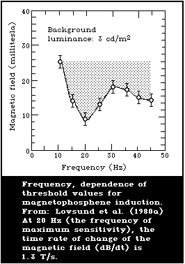 Another potentially important target of ELF magnetic field
interactions is the nervous system. From a consideration of the
naturally occurring fields in the central nervous system, Bernhardt
(1979) concluded that magnetic fields in the 1 - 100 Hz frequency
range, which can induce current densities in tissue of approximately
1 mA/m2 or less, should not have a direct effect on the brain's
electrical activity. The strength of a 60-Hz magnetic field that
would induce a peak current density of this magnitude in the
cranium of a human subject was calculated to be about 0.5 mT
(Tenforde, 1985a).
In a careful study on human perception to 60 Hz magnetic
fields, Tucker & Schmitt (1978) did not find any significantly
perceptive individuals among more than 200 subjects exposed to a
field with an amplitude of 2.1 mT. Several behavioural tests on
mice exposed to a 60-Hz magnetic field that induced a peak current
density approaching 1 mA/m2 in the peripheral cranial region also
yielded negative findings (Davis et al., 1984). The results of
these studies suggest that ELF magnetic fields must have
significantly greater amplitudes than the theoretically calculated
threshold values in order to perturb animal behaviour. However, it
is important to recognize the inherent deficiencies of a simple
theoretical model that treats the central nervous system as a
region of uniform conductivity. In addition, the induced current
in a loop of maximum radius at the brain's surface may not be the
relevant parameter to consider in predicting the response to ELF
magnetic fields. The regions of the central nervous system that
might be responsive to these fields may have significantly smaller
dimensions than the entire cranium. Thus, a large increase in the
ELF magnetic field strength would be necessary to evoke a
measurable electrical and/or behavioural perturbation.
It is reasonable to suppose that these effects result from the
interaction of the induced electric fields and currents with the
membranes of nerve and muscle cells, thereby causing changes in the
electrical excitability of these cells in the same way as naturally
occurring or directly applied electric fields.
The permeability to ions of the nerve (and muscle) cell
membranes depends on the membrane potential. It is this voltage-
dependent permeability that gives the cells the property of being
electrically excitable. When an electric field is applied, various
charged side-groups of certain proteins embedded in the membrane
change their configuration, thereby causing a larger structural
change in the protein as a whole. In this new conformation, ions
are able to pass through the membrane by binding temporarily with
the protein molecule at various sites, thus "hopping" through the
membrane. In any area of a membrane, there are a large number of
"gating" molecules, and the effect of an induced electric field may
involve an alteration in the proportion of gates that are open.
This type of interaction could significantly influence membrane
permeability.
In addition, there is a specific type of protein molecule for
each species of ion, permitting different ionic responses to the
same electric field. Thus, in response to a depolarizing electric
field, there is a large increase in Na+ permeability in the
membrane of a nerve cell tending to depolarize the cell further.
This event is followed by a slower change in K+ permeability and an
inactivation of the Na+ channel, resulting in a repolarization.
Induced fields sufficient to exceed a threshold depolarization
value can result in an action potential that is capable of
stimulating other excitable cells. These effects are well
understood. ELF magnetic fields inducing such large depolarizations
may result in nerve stimulation or muscle contraction, or even in
fibrillation. ELF magnetic fields inducing weak electric fields
may also interact with, or modulate, nervous system activity in a
manner that is less well understood. However, these interactions
can produce changes in electrical excitability. Such interactions
may be involved in, for example, magneto- or electrophosphenes.
The ELF field interactions described above exhibit frequency-
dependent thresholds characteristic of nervous tissue, and have
been well documented by Bernhardt (1979, 1985). This frequency
dependence is very important when relating experimental results
obtained using high frequencies or very short pulses to effects
anticipated at 50/60 Hz, at least as far as acute responses are
concerned. The main factors governing this dependence are
accommodation and ionic mobility. As a result, there is a
characteristic U-shaped dependence of threshold current density on
frequency, with the lowest values for most nervous tissues
occurring between 10 Hz and 100 kHz. At low frequencies, the
effects of accommodation predominate, which is thought to be
related to the slow inactivation of the Na+ channel. At higher
frequencies, the time available during each cycle for ions to
migrate across the membrane, an all or nothing event, becomes
limiting; direct electrical excitation gives way to heating
somewhere between 100 Hz and 300 kHz.
It should be noted that the theoretically calculated field
intensities at 20 Hz for stimulating the visual system are only
slightly lower than the perception threshold for magnetophosphenes
(Bernhardt, 1985). With regard to "hazardous values" and the upper
limit of the field strength that leads to injury, the ultimate
criterion for the definition of injury may be the initiation of
heart fibrillation. The threshold for extra-systole induction at
60 Hz is estimated to be above 300 mT for stimulation times of 1
second or longer, and the threshold for ventricular fibrillation is
higher by a factor of 3 - 5 (Bernhardt, 1985). For shorter
exposure times, higher field strengths are necessary to produce
similar biological effects.
Silny (1986) measured the stimulation threshold of the heart in
8 dogs exposed to time-varying magnetic fields. He converted the
thresholds found in dogs to the equivalent thresholds expected in
human beings. From his data, the fibrillation threshold for the
human heart was estimated to be 1 T at 50 Hz, for magnetic fields
acting perpendicular to the body axis.
4.3. Other Magnetic Field Interactions Under Study
The transduction mechanism for ELF magnetic fields described in
section 4.2 is supported by experimental data for electrically
excitable tissues. For other biological effects observed with ELF
fields that induce smaller current densities (below the level that
could significantly affect the cell membrane potential), other
transduction mechanisms have been proposed. For example, changes
in cell-surface receptor molecules and in ion binding to membrane
surfaces have been reported to occur, as a result of exposure to
ELF magnetic fields. It has been proposed that the pericellular
currents induced by an ELF field may produce electrochemical
alterations in components of the cell membrane surface. These
events, in turn, send signals across the cell membrane barrier that
produce alterations in intracellular biochemical and physiological
functions. This hypothesized scheme of transductive coupling
between induced electric currents in the extracellular medium and
the intracellular events occurring in living cells is illustrated
schematically in Fig. 6.
Another potentially important target of ELF magnetic field
interactions is the nervous system. From a consideration of the
naturally occurring fields in the central nervous system, Bernhardt
(1979) concluded that magnetic fields in the 1 - 100 Hz frequency
range, which can induce current densities in tissue of approximately
1 mA/m2 or less, should not have a direct effect on the brain's
electrical activity. The strength of a 60-Hz magnetic field that
would induce a peak current density of this magnitude in the
cranium of a human subject was calculated to be about 0.5 mT
(Tenforde, 1985a).
In a careful study on human perception to 60 Hz magnetic
fields, Tucker & Schmitt (1978) did not find any significantly
perceptive individuals among more than 200 subjects exposed to a
field with an amplitude of 2.1 mT. Several behavioural tests on
mice exposed to a 60-Hz magnetic field that induced a peak current
density approaching 1 mA/m2 in the peripheral cranial region also
yielded negative findings (Davis et al., 1984). The results of
these studies suggest that ELF magnetic fields must have
significantly greater amplitudes than the theoretically calculated
threshold values in order to perturb animal behaviour. However, it
is important to recognize the inherent deficiencies of a simple
theoretical model that treats the central nervous system as a
region of uniform conductivity. In addition, the induced current
in a loop of maximum radius at the brain's surface may not be the
relevant parameter to consider in predicting the response to ELF
magnetic fields. The regions of the central nervous system that
might be responsive to these fields may have significantly smaller
dimensions than the entire cranium. Thus, a large increase in the
ELF magnetic field strength would be necessary to evoke a
measurable electrical and/or behavioural perturbation.
It is reasonable to suppose that these effects result from the
interaction of the induced electric fields and currents with the
membranes of nerve and muscle cells, thereby causing changes in the
electrical excitability of these cells in the same way as naturally
occurring or directly applied electric fields.
The permeability to ions of the nerve (and muscle) cell
membranes depends on the membrane potential. It is this voltage-
dependent permeability that gives the cells the property of being
electrically excitable. When an electric field is applied, various
charged side-groups of certain proteins embedded in the membrane
change their configuration, thereby causing a larger structural
change in the protein as a whole. In this new conformation, ions
are able to pass through the membrane by binding temporarily with
the protein molecule at various sites, thus "hopping" through the
membrane. In any area of a membrane, there are a large number of
"gating" molecules, and the effect of an induced electric field may
involve an alteration in the proportion of gates that are open.
This type of interaction could significantly influence membrane
permeability.
In addition, there is a specific type of protein molecule for
each species of ion, permitting different ionic responses to the
same electric field. Thus, in response to a depolarizing electric
field, there is a large increase in Na+ permeability in the
membrane of a nerve cell tending to depolarize the cell further.
This event is followed by a slower change in K+ permeability and an
inactivation of the Na+ channel, resulting in a repolarization.
Induced fields sufficient to exceed a threshold depolarization
value can result in an action potential that is capable of
stimulating other excitable cells. These effects are well
understood. ELF magnetic fields inducing such large depolarizations
may result in nerve stimulation or muscle contraction, or even in
fibrillation. ELF magnetic fields inducing weak electric fields
may also interact with, or modulate, nervous system activity in a
manner that is less well understood. However, these interactions
can produce changes in electrical excitability. Such interactions
may be involved in, for example, magneto- or electrophosphenes.
The ELF field interactions described above exhibit frequency-
dependent thresholds characteristic of nervous tissue, and have
been well documented by Bernhardt (1979, 1985). This frequency
dependence is very important when relating experimental results
obtained using high frequencies or very short pulses to effects
anticipated at 50/60 Hz, at least as far as acute responses are
concerned. The main factors governing this dependence are
accommodation and ionic mobility. As a result, there is a
characteristic U-shaped dependence of threshold current density on
frequency, with the lowest values for most nervous tissues
occurring between 10 Hz and 100 kHz. At low frequencies, the
effects of accommodation predominate, which is thought to be
related to the slow inactivation of the Na+ channel. At higher
frequencies, the time available during each cycle for ions to
migrate across the membrane, an all or nothing event, becomes
limiting; direct electrical excitation gives way to heating
somewhere between 100 Hz and 300 kHz.
It should be noted that the theoretically calculated field
intensities at 20 Hz for stimulating the visual system are only
slightly lower than the perception threshold for magnetophosphenes
(Bernhardt, 1985). With regard to "hazardous values" and the upper
limit of the field strength that leads to injury, the ultimate
criterion for the definition of injury may be the initiation of
heart fibrillation. The threshold for extra-systole induction at
60 Hz is estimated to be above 300 mT for stimulation times of 1
second or longer, and the threshold for ventricular fibrillation is
higher by a factor of 3 - 5 (Bernhardt, 1985). For shorter
exposure times, higher field strengths are necessary to produce
similar biological effects.
Silny (1986) measured the stimulation threshold of the heart in
8 dogs exposed to time-varying magnetic fields. He converted the
thresholds found in dogs to the equivalent thresholds expected in
human beings. From his data, the fibrillation threshold for the
human heart was estimated to be 1 T at 50 Hz, for magnetic fields
acting perpendicular to the body axis.
4.3. Other Magnetic Field Interactions Under Study
The transduction mechanism for ELF magnetic fields described in
section 4.2 is supported by experimental data for electrically
excitable tissues. For other biological effects observed with ELF
fields that induce smaller current densities (below the level that
could significantly affect the cell membrane potential), other
transduction mechanisms have been proposed. For example, changes
in cell-surface receptor molecules and in ion binding to membrane
surfaces have been reported to occur, as a result of exposure to
ELF magnetic fields. It has been proposed that the pericellular
currents induced by an ELF field may produce electrochemical
alterations in components of the cell membrane surface. These
events, in turn, send signals across the cell membrane barrier that
produce alterations in intracellular biochemical and physiological
functions. This hypothesized scheme of transductive coupling
between induced electric currents in the extracellular medium and
the intracellular events occurring in living cells is illustrated
schematically in Fig. 6.
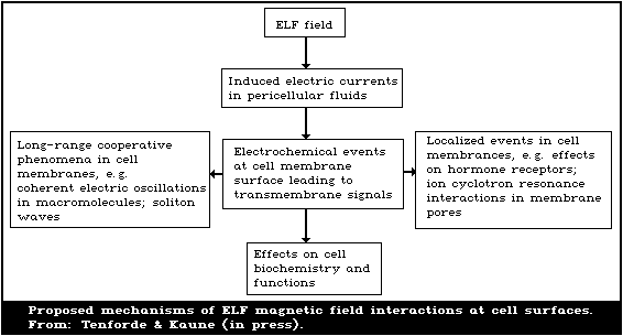 The key element in the sequence of events through which
externally applied ELF fields influence cellular properties is the
transductive signalling event within the cell membrane. Numerous
theoretical models have been proposed for the transmembrane
signalling process (or processes) that are triggered by induced
pericellular electric currents (Adey, 1980, 1981, 1983). In the
broadest sense, these hypothesized mechanisms can be grouped into
two general classes:
(a) long-range cooperative phenomena established within
the matrix of glycoproteins and lipoproteins that
constitute the cell membrane; and
(b) localized events occurring at specific ligand-binding
sites (receptors) at the outer membrane surface, or
events occurring within ion-selective channels that
span the membrane and electrically couple the
intracellular and extracellular fluids.
These classes of phenomena are depicted by the boxes at the left
and right sides of Fig. 6 and will be discussed separately.
4.3.1. Long-range cooperative phenomena in cell membranes
The electric fields induced in tissue by externally-applied
low-amplitude ELF electromagnetic fields are several orders of
magnitude less than the voltage gradient that exists across the
living cell membrane. It has therefore been proposed that the
cellular response to external ELF fields may involve an
amplification process in which a weak electric field induced in the
extracellular fluid acts as a "trigger" for the initiation of long-
range cooperative events within the cell membrane (Adey, 1981).
The basic premise underlying this theoretical concept is that the
cell membrane exists in a metastable, non-equilibrium state that
can be significantly perturbed by a weak electrical stimulus.
Various physical models of such interactions have generally treated
the cell membrane as a lattice in which nonlinear oscillations are
established by weak electrical (or electrochemical) stimuli. These
oscillations are amplified by the collective excitation of patches
of membrane molecules that extend over a significant portion of
the cell surface. The stored energy resulting from this collective
mode of molecular excitation is then released as metabolic chemical
energy through the activation of ion pumps or enzymatic reactions
within the membrane (Frohlich, 1968, 1977; Grodsky, 1976, 1977;
Kaczmarek, 1977; Lawrence & Adey, 1982, 1983; Adey, 1983).
4.3.2. Localized interactions of external ELF fields with
cell membrane structures
Recent experimental evidence and theoretical models have given
support to the concept that the interactions of ELF electromagnetic
fields with living cells occur at specific loci on the cell
membrane. In many ways, this concept is more attractive than the
hypothesized long-range membrane interactions described above.
Apart from the abstract nature of such theories, the concept of
long-range interactions that involve a large fraction of the cell
membrane surface is generally feasible only for electromagnetic
fields with frequencies well above the ELF range. Recent
theoretical efforts have therefore focused on the possibility that
weak ELF field interactions could significantly alter either
ligand-receptor interactions at the membrane surface, or the
transmembrane movement of electrolytes. Theoretical and
experimental developments in this area include the following:
(a) Ligand-receptor interactions
Chiabrera et al. (1984) proposed a model of membrane
interactions in which a microelectrophoretic motion induced in
the cell membrane by weak ELF electric fields influences the
average distance between charged ligands and the cell-surface
receptors to which they are bound. In this theoretical model,
the effect of the imposed electric field is to decrease the
mean lifetime of the ligand-receptor complexes on the membrane
surface. The authors propose that this effect could influence
various biological phenomena such as the activation of
lymphocytes by antigens and various lectins. An ELF field
interaction of this type could also influence the gating
mechanisms that control the membrane transport of various types
of cations such as calcium.
(b) Combined static and ELF field interactions
Some experimental evidence suggests that ion cyclotron
resonance effects could occur between ELF fields and static
magnetic fields with intensities comparable to that of the
geomagnetic field. Briefly summarized, it has been reported
that magnetic resonance conditions influence the dielectric
properties and growth rate of yeast cells (Jafary-Asl et al.,
1982), the rate of lysozyme reaction with a cell membrane
substrate (Jafary-Asl et al., 1982), the behaviour of rats in a
timing discrimination task (Liboff et al., 1985), and the rate
of calcium ion release from the surfaces of brain cells exposed
in vitro to low-intensity electromagnetic fields (Blackman et
al., 1985a,b). The first two of these biological effects were
claimed to occur in response to conventional nuclear magnetic
resonance conditions under which the static field intensity and
the frequency of the electromagnetic field were related by the
Larmor relationship for various nuclei, including 1H, 23Na,
31P, 35Cl, and 39K (Jafary-Asl et al., 1982). In a third study
(Liboff et al., 1985), reversible changes in rodent timing
behaviour were observed when rats were simultaneously exposed
to a horizontal 60-Hz magnetic field and a vertical
magnetostatic field with a flux density of 26 µT. This
combination of static field intensity and oscillating field
frequency satisfies the cyclotron resonance conditions for
lithium ions, which are thought to exert neuropharmacological
effects. In the fourth study (Blackman et al., 1985b), a
generalized relationship was derived between the biologically
effective electromagnetic field frequency and the static
magnetic field flux density. This relationship established a
proportionality between the frequency of the oscillating field
and the static magnetic field flux density multiplied by an
index, (2n + 1), where n = 0 or 1.
Liboff (1985) proposed that these weak interactions, which
involve energy transfer from the external field that is 8 orders of
magnitude less than the Boltzmann thermal energy (kT), could
nevertheless impart kinetic energy to ions, such as calcium, moving
through transmembrane channels. The theoretical argument was made
by McLeod & Liboff (1986) that ion channels provide an environment
in which damping effects on ion motion due to collision may be
reduced relative to the high collision frequencies that exist in
bulk aqueous media. Nevertheless, a simple calculation indicates
that, under the various experimental conditions described above,
the induced electric field within ion transport channels is of the
order of 10-10 V/m. This field level is 2 orders of magnitude less
than the Nyquist thermoelectric noise present in membrane channels
(Bawin & Adey, 1976). Overall, the experimental data that suggest
a possible role of cyclotron resonance effects on ion binding to
membrane surfaces and on cation transport through cell membrane
pores are intriguing, but there is a clear need for refinements in
the theoretical description of this phenomenon and to substantiate
the experimental results.
5. EXPERIMENTAL DATA ON THE BIOLOGICAL EFFECTS OF STATIC MAGNETIC FIELDS
In this section, the aim is to present a review of experimental
observations on the biological effects of exposure to magnetic
fields, and to relate them to data presented in the preceding
section, in which the mechanisms of interaction were discussed.
Empirical observations for which no theoretical explanations are
available, at present, will be pointed out, and an attempt will be
made to identify gaps in knowledge. The data discussed here were
selected on the basis of their relevance for the assessment of
health risks. Thus, many papers have been omitted from the
discussion.
Several comprehensive sources of experimental data on the
biological effects of magnetic fields are available. Older results
have been collected in two volumes edited by Barnothy, M.F., ed.
(1964, 1969) and the monograph by Kholodov (1966, 1974); more
recent results can be found in the report of the American Institute
of Biological Sciences (1985). Some recent reviews include those
prepared by Bogolyubov (1981), Kholodov (1982), Schulten (1982),
Galaktionova et al. (1985), Sidjakin (in press), Tenforde (1979,
1985a,b,c, 1986a), and Tenforde et al. (1985). Valuable information
and extensive bibliographies can be found in review papers by
Budinger (1979, 1981), Budinger & Collander (1983), Persson &
Stahlberg (1984), and Tenforde & Budinger (1986), which address the
biological effects of magnetic fields in the context of the safety
of magnetic resonance imaging and in vivo spectroscopy.
All the above reviews are concerned with potential risks for
human health from exposure to magnetic fields of a strength greater
than that of the geomagnetic field. This document does not deal
with magnetic fields of a strength below that of the geomagnetic
field. However, readers interested in this aspect are referred to
reviews by Nakhil'nitskaya et al. (1978) and Kopanov & Shakula
(1985).
The organization of this section will follow the order of
increasing biological complexity of the system studied.
5.1. Molecular Interactions
Research on magnetic field interactions with biological
molecules has led to a diversity of findings as exemplified by the
results of studies on various enzymes summarized in Table 8. A
total of 15 reports has appeared in which the reaction rates of 17
different enzymes were studied during exposure to stationary
magnetic fields over a broad range of field strengths, and with
widely varying exposure times, reaction temperatures and pH levels,
and conditions of field uniformity. Overall, 58% of the
experimental studies showed no effects of the field exposure, while
33% and 8% of the tests showed increases and decreases,
respectively, in the rate of enzyme reactions in the exposed
samples relative to controls. As discussed earlier in section 4,
in certain systems, such as enzymes that involve radical
intermediate stages as part of their reaction pathways, it might be
anticipated that the reaction would be sensitive to the presence of
a magnetic field. However, for several other enzyme systems there
is no obvious physical mechanism that could explain the observed
magnetic sensitivity at the field intensities that were used. It
is interesting to note, for example, that Cook & Smith (1964) found
that the activity of trypsin increased by up to 23% during a 2-h
exposure to a 0.8-T field, whereas Vajda (1980) and Nazarova et al.
(1982) did not observe any change in enzyme activity during
exposures of 2-8 h duration in a 1.4-T field. Furthermore,
Nazarova et al. (1982) found that trypsin activity was not affected
by a 2.5 h exposure to a 10-T field, and Rabinovitch et al.
(1967a,b) did not observe any change in trypsin activity either
during a 9 min exposure to a 22-T field, or following a 3.7 h
pretreatment of the enzyme in a 20.8-T field.
Another aspect of the data presented in Table 8 that merits
comment is the finding in two different laboratories of an increase
in the reaction rate of the metalloenzyme catalase in response to
exposure to a magnetic field (Haberditzl, 1967; Vainer et al.,
1978). Vainer et al. (1978) reported that the reaction rate of
catalase varied linearly with field between 0 and 0.8 T, increasing
by 20% at 0.8 T. The action of this enzyme may involve a radical
intermediate state which, as discussed in the preceeding section,
might be anticipated to exhibit magnetic sensitivity. Several
other biologically important enzymes that may have radical
intermediate steps in their pathways include the cytochrome P-450
enzymes, which are involved in steroid hormone metabolism, and
lipoxygenase and cyclo-oxygenase, both of which are involved in the
synthesis of prostaglandins (Saunders & Cass, 1983). Further
studies on these enzyme systems would provide useful insight into
whether enzymatic pathways that involve radical intermediate states
exhibit sensitivity to a stationary magnetic field, with possible
consequences for cellular and tissue functions (Schulten, 1986).
A well-studied mechanism by which static magnetic fields can
influence macromolecules is through a magneto-orientational effect.
As discussed in section 4, this phenomenon produces measurable
effects on single molecules, only at field strengths greater than
10 T. Various macromolecular assemblies, such as retinal
photopigments, can be oriented in fields of less than 1 T.
However, at present, there are no data suggesting that magneto-
orientation of these various macromolecules exerts profound effects
on vital membrane, cellular, or tissue function. For example,
mammalian visual functions have been found to be unaffected by
static magnetic fields up to 1.5 T (Gaffey & Tenforde, 1984).
Table 8. Magnetic field effects on enzyme systems
-------------------------------------------------------------------
Enzyme Applied Effect on Reference
field enzyme
strength activity
(tesla)
-------------------------------------------------------------------
Acetylcholinesterase 1.7 increase Young (1969)
Alcohol dehydrogenase 1.4 none Muller et al. (1971)
Aldolase 17 none Rabinovitch et al.
(1967a,b)
Asparaginase 1.7 increase Shishlo (1974)
beta-galactosidase 1 none Thomas & Morris
(1981)
Carboxydismutase 2 increase Akoyunoglou (1964)
Catalase 6 increase Haberditzl (1967)
Catalase 0.8 increase Vainer et al. (1978)
Cytochrome oxidase 1.3 increase Gorczynska et al.
(1982)
DNase 0.3 increase Komolova et al.
(1972)
Glumatic dehydrogenase 7.8 decrease Haberditzl (1967)
Histidase 1.7 decrease Shishlo (1974)
Lactic dehydrogenase 1.4 none Muller et al. (1971)
Peroxidase 17 none Rabinovitch et al.
(1967a,b)
RNase 17 none Rabinovitch et al.
(1967a,b)
RNase 4.8 none Maling et al. (1965)
RNase 1.4 none Muller et al. (1971)
RNase 0.3 none Komolova et al.
(1972)
Succinate-cytochrome-C
reductase 4.8 none Maling et al. (1965)
Trypsin 0.8 increase Cook & Smith (1964)
Trypsin 20.8 none Rabinovitch et al.
(1967a,b)
Trypsin 10 none Nazarova et al.
(1982)
Trypsin 1.4 none Vajda (1980)
Tryosinase 17 none Rabinovitch et al.
(1967a,b)
-------------------------------------------------------------------
5.2. Effects at the Cell Level
The results of a number of studies conducted in the 1960s and
earlier suggested that exposure to stationary fields might lead to
physiological, morphological, and growth abnormalities at the
cellular level (Barnothy, M.F., 1964, 1969). Degenerative changes
such as pycnosis (Mulay & Mulay, 1961; Pereira et al., 1967),
decreased DNA synthesis (D'Souza et al., 1969) and growth
inhibition (Gerencer et al., 1962; Butler & Dean, 1964) were noted
for various types of normal and tumour cells. In contrast to these
observations, a large number of more recent studies using magnetic
field intensities and exposure times that were equal to or greater
than those used in the earlier work have failed to produce effects
on cell growth (Montgomery & Smith, 1963; Halpern & Greene, 1964;
Hall et al., 1964; Rockwell, 1977; Iwasaki et al., 1978; Frazier et
al., 1979, Nath et al., 1980). It is also interesting to note that
early reports (Barnothy, J.M., 1964; Gross, 1964) of in vivo
tumour growth inhibition by stationary magnetic fields have not
been replicated in other studies (Eiselein et al., 1961; Chandra &
Stefani, 1979). All of the studies mentioned above were performed
under different exposure conditions and thus are difficult to
compare.
Malinin et al. (1976) reported that exposure of human WI-38
fibroblasts and murine L-929 cells to a 0.5-T field for 4-8 h at
4 °K led to subsequent growth inhibition compared with controls, when
the cells were thawed and cultured at 30 °C. The exposed cultures
also appeared to undergo morphological transformation and to lose
sensitivity to contact inhibition of cell division in long-term
cultures. These observations were later shown to be the result of
using unconventional culture techniques in which control cells were
subcultured at 5- to 6-day intervals, while cultures grown from
exposed cells were only passaged at 28- to 45-day intervals. When
Frazier et al. (1979) used similar culture techniques, they were
able to replicate, in unexposed cultures of WI-38 and L-929 cells,
the morphological transformation that had been reported by Malinin
et al. (1976) to result from magnetic field exposure. Thus, the
results of Malinin et al. (1976) should be discounted in an
evaluation of magnetic field effects on cell cultures.
Although the preponderance of available experimental evidence
indicates that stationary magnetic fields with intensities up to 2
T exert little influence on cell growth properties, there are
potential mechanisms, discussed by Tenforde (1985b), by means of
which effects might occur. These include:
(a) Enzymatic pathways that contain radical intermediate stages
and may be sensitive to the presence of strong magnetic
fields;
(b) The redistribution of paramagnetic oxygen molecules in the
presence of a strong magnetic field gradient (Aceto et al.,
1970). The magnetomechanical movement of dissolved oxygen
in an aqueous medium has been demonstrated experimentally
(Lyu et al., 1978; Ueno & Harada, 1982), but, as yet, there
are no clear tests of the potential biological consequences
of this effect.
(c) As the lamellar phospholipids of cell membranes are
diamagnetically anisotropic, the orientational effect of an
applied magnetic field exceeding approximately 0.1 - 1 T
could significantly perturb membrane transport properties
(Labes, 1966). In support of this proposal, direct
evidence has been obtained for magnetic field effects on
the diffusional properties of liquid crystals (Teucher et
al., 1971; Hakemi & Labes, 1974, 1975). Using measured
values for the anisotropic diamagnetic susceptibility of
model phospholipid membranes (Boroske & Helfrich, 1978),
it can be estimated from theoretical considerations that
the magnetic interaction energy within a typical cell
membrane will exceed the Boltzmann thermal energy, kT, in
stationary fields greater than approximately 0.5 T
(Tenforde, 1985b). At sufficiently high magnetic field
intensities, a perturbation of membrane properties might
therefore be expected to occur, with possible consequences
for other cellular functions.
(d) The sensitivity of cell membranes to magnetic field
interactions may be greatest at phase transition
temperatures (Amer, 1965; Aceto et al., 1970). This
hypothesis is based on the concept that perturbations
introduced by relatively weak magnetic interactions should
be amplified near a phase transition temperature at which
membrane properties undergo abrupt changes. Some indirect
support for this hypothesis was obtained from studies on
thermally-induced developmental failure in flour beetles
(Amer, 1965), in which higher temperatures were required to
elicit developmental wing abnormalities in the presence of
a strong magnetic field. More direct evidence for membrane
sensitivity to static magnetic fields at phase transition
temperatures has recently been obtained (Liburdy et al.,
1986; Liburdy & Tenforde, 1986). These investigators
observed changes in the permeability of liposome bilayer
membranes composed of saturated phospholipids, when the
liposomes were exposed to static magnetic fields at
temperatures in the prephase transition region from 40 to
40.7 °C. At temperatures of lower than 40 °C or higher than
40.7 °C, no effects on liposome membrane transport were
observed in fields as high as 7.5 T.
5.3. Effects on Organs and Tissues
Examples of mammalian tissue and organ alterations that have
been observed following magnetic field exposure include changes in:
(a) blood and bone marrow cellular composition (Barnothy
et al., 1956; Barnothy & Sumegi, 1969a,b; Nakagawa et
al. 1980; Gorchonskaya, 1984);
(b) serum chemistry (Nakagawa et al. 1980; Tvildiani et
al. 1983);
(c) microcirculation (Demetsky et al., 1979; Grohmann et
al., 1986)
(d) thrombocyte coagulation (Rusyayev, 1979);
(e) electrolyte balance in blood, urine, and various
tissues (Hanneman, 1969; Markuze et al., 1973;
Tvildiani et al., 1981);
(f) functional and structural properties of various
organs and tissues (Reno & Nutini, 1963, 1964;
Toroptsev, 1968; Galaktionova & Strzhizhovsky, 1973;
Bucking et al., 1974; Wordsworth, 1974; Kholodov &
Shishlo, 1980; Strzhizhovsky et al., 1980; Rabino-
vitch et al., 1983; Strzhizhovsky & Mastryukova,
1983);
(g) immune response (Pautrizel et al., 1969; Kandil &
Elashmawy, 1981); and
(h) endocrine regulation (Klimovskaya & Maslova, 1981,
1983; Friedman & Carey, 1972).
With the exception of one study on endocrine changes
(Klimovskaya & Maslova, 1983), all of the reported alterations in
tissue and organ properties were observed at static magnetic field
levels below 1 T. These observations are therefore difficult to
reconcile with the growing body of evidence that the development,
growth, and homeostatic regulation of mammals is not significantly
affected by prolonged exposure to fields of this magnitude.
Many of the experimental reports have been based on studies
with small numbers of exposed and control subjects, and often no
attempt has been made by the investigators to replicate their
experimental results. Furthermore, the magnetic field exposure
conditions frequently have not been well documented. In some
studies, inadequate controls were used, such as the use of cage-
control animals, instead of sham-exposed controls. In this case,
effects attributed to magnetic fields may have occurred in response
to stresses imposed by other factors, such as adaptation to new
caging conditions, differences in ambient temperature, sound
levels, lighting conditions, and so forth. There have been few
attempts to verify the findings of tissue and organ effects through
independent replication in other laboratories. In the few cases
where such attempts have been made, the original results have not
been successfully replicated. For example, the early reports
(Barnothy et al., 1956; Barnothy & Sumegi, 1969a,b; Nakagawa et
al., 1980) of haematopoietic alterations have not been confirmed in
other studies (Eiselein et al., 1961; Nahas et al., 1975; Viktova
et al., 1976; Battocletti et al., 1981). Similarly, earlier
reports (Pautrizel et al., 1969; Kandil & Elashmawy, 1981) that
magnetic fields alter the immune status of exposed subjects have
not been confirmed by Bellossi (1983) or in more recent studies
designed to test humoral and cell-mediated immunity in mice exposed
for 6 days to a 1.5-T stationary magnetic field (Tenforde &
Shifrine, 1984).
It should be added that, where effects have been identified,
efforts have seldom been made to explore the consequences for other
related end-points, as a means of verifying the previous findings.
Furthermore, only a few studies have addressed magnetic field
effects on tissues and organs using classical anatomical and
physiological methods. In view of these considerations, the
existence of deleterious effects of static magnetic fields on
tissue and organ functions must, at present, be considered as
questionable.
5.4. Effects on the Circulatory System
The occurrence of magnetically induced potentials associated
with blood flow in the aorta (Fig. 4, section 4.1) has been
demonstrated on electrocardiogram (ECG) recordings from rats
(Gaffey & Tenforde, 1981), rabbits (Togawa et al., 1967), dogs and
baboons (Gaffey & Tenforde 1979; Gaffey et al., 1980), and monkeys
(Beischer & Knepton, 1964; Beischer, 1969; Tenforde et al., 1983)
exposed to static magnetic fields (Fig. 7). The primary change in
the ECG in the field is an alteration of the signal amplitude at
the locus of the T-wave. The repolarization of ventricular heart
muscle, which gives rise to the T-wave, occurs in the normal ECG at
approximately the same time in the cardiac cycle as the ejection of
blood into the aorta. It is therefore reasonable to expect that
the flow potential induced by the magnetic field is superimposed on
the T-wave.
The key element in the sequence of events through which
externally applied ELF fields influence cellular properties is the
transductive signalling event within the cell membrane. Numerous
theoretical models have been proposed for the transmembrane
signalling process (or processes) that are triggered by induced
pericellular electric currents (Adey, 1980, 1981, 1983). In the
broadest sense, these hypothesized mechanisms can be grouped into
two general classes:
(a) long-range cooperative phenomena established within
the matrix of glycoproteins and lipoproteins that
constitute the cell membrane; and
(b) localized events occurring at specific ligand-binding
sites (receptors) at the outer membrane surface, or
events occurring within ion-selective channels that
span the membrane and electrically couple the
intracellular and extracellular fluids.
These classes of phenomena are depicted by the boxes at the left
and right sides of Fig. 6 and will be discussed separately.
4.3.1. Long-range cooperative phenomena in cell membranes
The electric fields induced in tissue by externally-applied
low-amplitude ELF electromagnetic fields are several orders of
magnitude less than the voltage gradient that exists across the
living cell membrane. It has therefore been proposed that the
cellular response to external ELF fields may involve an
amplification process in which a weak electric field induced in the
extracellular fluid acts as a "trigger" for the initiation of long-
range cooperative events within the cell membrane (Adey, 1981).
The basic premise underlying this theoretical concept is that the
cell membrane exists in a metastable, non-equilibrium state that
can be significantly perturbed by a weak electrical stimulus.
Various physical models of such interactions have generally treated
the cell membrane as a lattice in which nonlinear oscillations are
established by weak electrical (or electrochemical) stimuli. These
oscillations are amplified by the collective excitation of patches
of membrane molecules that extend over a significant portion of
the cell surface. The stored energy resulting from this collective
mode of molecular excitation is then released as metabolic chemical
energy through the activation of ion pumps or enzymatic reactions
within the membrane (Frohlich, 1968, 1977; Grodsky, 1976, 1977;
Kaczmarek, 1977; Lawrence & Adey, 1982, 1983; Adey, 1983).
4.3.2. Localized interactions of external ELF fields with
cell membrane structures
Recent experimental evidence and theoretical models have given
support to the concept that the interactions of ELF electromagnetic
fields with living cells occur at specific loci on the cell
membrane. In many ways, this concept is more attractive than the
hypothesized long-range membrane interactions described above.
Apart from the abstract nature of such theories, the concept of
long-range interactions that involve a large fraction of the cell
membrane surface is generally feasible only for electromagnetic
fields with frequencies well above the ELF range. Recent
theoretical efforts have therefore focused on the possibility that
weak ELF field interactions could significantly alter either
ligand-receptor interactions at the membrane surface, or the
transmembrane movement of electrolytes. Theoretical and
experimental developments in this area include the following:
(a) Ligand-receptor interactions
Chiabrera et al. (1984) proposed a model of membrane
interactions in which a microelectrophoretic motion induced in
the cell membrane by weak ELF electric fields influences the
average distance between charged ligands and the cell-surface
receptors to which they are bound. In this theoretical model,
the effect of the imposed electric field is to decrease the
mean lifetime of the ligand-receptor complexes on the membrane
surface. The authors propose that this effect could influence
various biological phenomena such as the activation of
lymphocytes by antigens and various lectins. An ELF field
interaction of this type could also influence the gating
mechanisms that control the membrane transport of various types
of cations such as calcium.
(b) Combined static and ELF field interactions
Some experimental evidence suggests that ion cyclotron
resonance effects could occur between ELF fields and static
magnetic fields with intensities comparable to that of the
geomagnetic field. Briefly summarized, it has been reported
that magnetic resonance conditions influence the dielectric
properties and growth rate of yeast cells (Jafary-Asl et al.,
1982), the rate of lysozyme reaction with a cell membrane
substrate (Jafary-Asl et al., 1982), the behaviour of rats in a
timing discrimination task (Liboff et al., 1985), and the rate
of calcium ion release from the surfaces of brain cells exposed
in vitro to low-intensity electromagnetic fields (Blackman et
al., 1985a,b). The first two of these biological effects were
claimed to occur in response to conventional nuclear magnetic
resonance conditions under which the static field intensity and
the frequency of the electromagnetic field were related by the
Larmor relationship for various nuclei, including 1H, 23Na,
31P, 35Cl, and 39K (Jafary-Asl et al., 1982). In a third study
(Liboff et al., 1985), reversible changes in rodent timing
behaviour were observed when rats were simultaneously exposed
to a horizontal 60-Hz magnetic field and a vertical
magnetostatic field with a flux density of 26 µT. This
combination of static field intensity and oscillating field
frequency satisfies the cyclotron resonance conditions for
lithium ions, which are thought to exert neuropharmacological
effects. In the fourth study (Blackman et al., 1985b), a
generalized relationship was derived between the biologically
effective electromagnetic field frequency and the static
magnetic field flux density. This relationship established a
proportionality between the frequency of the oscillating field
and the static magnetic field flux density multiplied by an
index, (2n + 1), where n = 0 or 1.
Liboff (1985) proposed that these weak interactions, which
involve energy transfer from the external field that is 8 orders of
magnitude less than the Boltzmann thermal energy (kT), could
nevertheless impart kinetic energy to ions, such as calcium, moving
through transmembrane channels. The theoretical argument was made
by McLeod & Liboff (1986) that ion channels provide an environment
in which damping effects on ion motion due to collision may be
reduced relative to the high collision frequencies that exist in
bulk aqueous media. Nevertheless, a simple calculation indicates
that, under the various experimental conditions described above,
the induced electric field within ion transport channels is of the
order of 10-10 V/m. This field level is 2 orders of magnitude less
than the Nyquist thermoelectric noise present in membrane channels
(Bawin & Adey, 1976). Overall, the experimental data that suggest
a possible role of cyclotron resonance effects on ion binding to
membrane surfaces and on cation transport through cell membrane
pores are intriguing, but there is a clear need for refinements in
the theoretical description of this phenomenon and to substantiate
the experimental results.
5. EXPERIMENTAL DATA ON THE BIOLOGICAL EFFECTS OF STATIC MAGNETIC FIELDS
In this section, the aim is to present a review of experimental
observations on the biological effects of exposure to magnetic
fields, and to relate them to data presented in the preceding
section, in which the mechanisms of interaction were discussed.
Empirical observations for which no theoretical explanations are
available, at present, will be pointed out, and an attempt will be
made to identify gaps in knowledge. The data discussed here were
selected on the basis of their relevance for the assessment of
health risks. Thus, many papers have been omitted from the
discussion.
Several comprehensive sources of experimental data on the
biological effects of magnetic fields are available. Older results
have been collected in two volumes edited by Barnothy, M.F., ed.
(1964, 1969) and the monograph by Kholodov (1966, 1974); more
recent results can be found in the report of the American Institute
of Biological Sciences (1985). Some recent reviews include those
prepared by Bogolyubov (1981), Kholodov (1982), Schulten (1982),
Galaktionova et al. (1985), Sidjakin (in press), Tenforde (1979,
1985a,b,c, 1986a), and Tenforde et al. (1985). Valuable information
and extensive bibliographies can be found in review papers by
Budinger (1979, 1981), Budinger & Collander (1983), Persson &
Stahlberg (1984), and Tenforde & Budinger (1986), which address the
biological effects of magnetic fields in the context of the safety
of magnetic resonance imaging and in vivo spectroscopy.
All the above reviews are concerned with potential risks for
human health from exposure to magnetic fields of a strength greater
than that of the geomagnetic field. This document does not deal
with magnetic fields of a strength below that of the geomagnetic
field. However, readers interested in this aspect are referred to
reviews by Nakhil'nitskaya et al. (1978) and Kopanov & Shakula
(1985).
The organization of this section will follow the order of
increasing biological complexity of the system studied.
5.1. Molecular Interactions
Research on magnetic field interactions with biological
molecules has led to a diversity of findings as exemplified by the
results of studies on various enzymes summarized in Table 8. A
total of 15 reports has appeared in which the reaction rates of 17
different enzymes were studied during exposure to stationary
magnetic fields over a broad range of field strengths, and with
widely varying exposure times, reaction temperatures and pH levels,
and conditions of field uniformity. Overall, 58% of the
experimental studies showed no effects of the field exposure, while
33% and 8% of the tests showed increases and decreases,
respectively, in the rate of enzyme reactions in the exposed
samples relative to controls. As discussed earlier in section 4,
in certain systems, such as enzymes that involve radical
intermediate stages as part of their reaction pathways, it might be
anticipated that the reaction would be sensitive to the presence of
a magnetic field. However, for several other enzyme systems there
is no obvious physical mechanism that could explain the observed
magnetic sensitivity at the field intensities that were used. It
is interesting to note, for example, that Cook & Smith (1964) found
that the activity of trypsin increased by up to 23% during a 2-h
exposure to a 0.8-T field, whereas Vajda (1980) and Nazarova et al.
(1982) did not observe any change in enzyme activity during
exposures of 2-8 h duration in a 1.4-T field. Furthermore,
Nazarova et al. (1982) found that trypsin activity was not affected
by a 2.5 h exposure to a 10-T field, and Rabinovitch et al.
(1967a,b) did not observe any change in trypsin activity either
during a 9 min exposure to a 22-T field, or following a 3.7 h
pretreatment of the enzyme in a 20.8-T field.
Another aspect of the data presented in Table 8 that merits
comment is the finding in two different laboratories of an increase
in the reaction rate of the metalloenzyme catalase in response to
exposure to a magnetic field (Haberditzl, 1967; Vainer et al.,
1978). Vainer et al. (1978) reported that the reaction rate of
catalase varied linearly with field between 0 and 0.8 T, increasing
by 20% at 0.8 T. The action of this enzyme may involve a radical
intermediate state which, as discussed in the preceeding section,
might be anticipated to exhibit magnetic sensitivity. Several
other biologically important enzymes that may have radical
intermediate steps in their pathways include the cytochrome P-450
enzymes, which are involved in steroid hormone metabolism, and
lipoxygenase and cyclo-oxygenase, both of which are involved in the
synthesis of prostaglandins (Saunders & Cass, 1983). Further
studies on these enzyme systems would provide useful insight into
whether enzymatic pathways that involve radical intermediate states
exhibit sensitivity to a stationary magnetic field, with possible
consequences for cellular and tissue functions (Schulten, 1986).
A well-studied mechanism by which static magnetic fields can
influence macromolecules is through a magneto-orientational effect.
As discussed in section 4, this phenomenon produces measurable
effects on single molecules, only at field strengths greater than
10 T. Various macromolecular assemblies, such as retinal
photopigments, can be oriented in fields of less than 1 T.
However, at present, there are no data suggesting that magneto-
orientation of these various macromolecules exerts profound effects
on vital membrane, cellular, or tissue function. For example,
mammalian visual functions have been found to be unaffected by
static magnetic fields up to 1.5 T (Gaffey & Tenforde, 1984).
Table 8. Magnetic field effects on enzyme systems
-------------------------------------------------------------------
Enzyme Applied Effect on Reference
field enzyme
strength activity
(tesla)
-------------------------------------------------------------------
Acetylcholinesterase 1.7 increase Young (1969)
Alcohol dehydrogenase 1.4 none Muller et al. (1971)
Aldolase 17 none Rabinovitch et al.
(1967a,b)
Asparaginase 1.7 increase Shishlo (1974)
beta-galactosidase 1 none Thomas & Morris
(1981)
Carboxydismutase 2 increase Akoyunoglou (1964)
Catalase 6 increase Haberditzl (1967)
Catalase 0.8 increase Vainer et al. (1978)
Cytochrome oxidase 1.3 increase Gorczynska et al.
(1982)
DNase 0.3 increase Komolova et al.
(1972)
Glumatic dehydrogenase 7.8 decrease Haberditzl (1967)
Histidase 1.7 decrease Shishlo (1974)
Lactic dehydrogenase 1.4 none Muller et al. (1971)
Peroxidase 17 none Rabinovitch et al.
(1967a,b)
RNase 17 none Rabinovitch et al.
(1967a,b)
RNase 4.8 none Maling et al. (1965)
RNase 1.4 none Muller et al. (1971)
RNase 0.3 none Komolova et al.
(1972)
Succinate-cytochrome-C
reductase 4.8 none Maling et al. (1965)
Trypsin 0.8 increase Cook & Smith (1964)
Trypsin 20.8 none Rabinovitch et al.
(1967a,b)
Trypsin 10 none Nazarova et al.
(1982)
Trypsin 1.4 none Vajda (1980)
Tryosinase 17 none Rabinovitch et al.
(1967a,b)
-------------------------------------------------------------------
5.2. Effects at the Cell Level
The results of a number of studies conducted in the 1960s and
earlier suggested that exposure to stationary fields might lead to
physiological, morphological, and growth abnormalities at the
cellular level (Barnothy, M.F., 1964, 1969). Degenerative changes
such as pycnosis (Mulay & Mulay, 1961; Pereira et al., 1967),
decreased DNA synthesis (D'Souza et al., 1969) and growth
inhibition (Gerencer et al., 1962; Butler & Dean, 1964) were noted
for various types of normal and tumour cells. In contrast to these
observations, a large number of more recent studies using magnetic
field intensities and exposure times that were equal to or greater
than those used in the earlier work have failed to produce effects
on cell growth (Montgomery & Smith, 1963; Halpern & Greene, 1964;
Hall et al., 1964; Rockwell, 1977; Iwasaki et al., 1978; Frazier et
al., 1979, Nath et al., 1980). It is also interesting to note that
early reports (Barnothy, J.M., 1964; Gross, 1964) of in vivo
tumour growth inhibition by stationary magnetic fields have not
been replicated in other studies (Eiselein et al., 1961; Chandra &
Stefani, 1979). All of the studies mentioned above were performed
under different exposure conditions and thus are difficult to
compare.
Malinin et al. (1976) reported that exposure of human WI-38
fibroblasts and murine L-929 cells to a 0.5-T field for 4-8 h at
4 °K led to subsequent growth inhibition compared with controls, when
the cells were thawed and cultured at 30 °C. The exposed cultures
also appeared to undergo morphological transformation and to lose
sensitivity to contact inhibition of cell division in long-term
cultures. These observations were later shown to be the result of
using unconventional culture techniques in which control cells were
subcultured at 5- to 6-day intervals, while cultures grown from
exposed cells were only passaged at 28- to 45-day intervals. When
Frazier et al. (1979) used similar culture techniques, they were
able to replicate, in unexposed cultures of WI-38 and L-929 cells,
the morphological transformation that had been reported by Malinin
et al. (1976) to result from magnetic field exposure. Thus, the
results of Malinin et al. (1976) should be discounted in an
evaluation of magnetic field effects on cell cultures.
Although the preponderance of available experimental evidence
indicates that stationary magnetic fields with intensities up to 2
T exert little influence on cell growth properties, there are
potential mechanisms, discussed by Tenforde (1985b), by means of
which effects might occur. These include:
(a) Enzymatic pathways that contain radical intermediate stages
and may be sensitive to the presence of strong magnetic
fields;
(b) The redistribution of paramagnetic oxygen molecules in the
presence of a strong magnetic field gradient (Aceto et al.,
1970). The magnetomechanical movement of dissolved oxygen
in an aqueous medium has been demonstrated experimentally
(Lyu et al., 1978; Ueno & Harada, 1982), but, as yet, there
are no clear tests of the potential biological consequences
of this effect.
(c) As the lamellar phospholipids of cell membranes are
diamagnetically anisotropic, the orientational effect of an
applied magnetic field exceeding approximately 0.1 - 1 T
could significantly perturb membrane transport properties
(Labes, 1966). In support of this proposal, direct
evidence has been obtained for magnetic field effects on
the diffusional properties of liquid crystals (Teucher et
al., 1971; Hakemi & Labes, 1974, 1975). Using measured
values for the anisotropic diamagnetic susceptibility of
model phospholipid membranes (Boroske & Helfrich, 1978),
it can be estimated from theoretical considerations that
the magnetic interaction energy within a typical cell
membrane will exceed the Boltzmann thermal energy, kT, in
stationary fields greater than approximately 0.5 T
(Tenforde, 1985b). At sufficiently high magnetic field
intensities, a perturbation of membrane properties might
therefore be expected to occur, with possible consequences
for other cellular functions.
(d) The sensitivity of cell membranes to magnetic field
interactions may be greatest at phase transition
temperatures (Amer, 1965; Aceto et al., 1970). This
hypothesis is based on the concept that perturbations
introduced by relatively weak magnetic interactions should
be amplified near a phase transition temperature at which
membrane properties undergo abrupt changes. Some indirect
support for this hypothesis was obtained from studies on
thermally-induced developmental failure in flour beetles
(Amer, 1965), in which higher temperatures were required to
elicit developmental wing abnormalities in the presence of
a strong magnetic field. More direct evidence for membrane
sensitivity to static magnetic fields at phase transition
temperatures has recently been obtained (Liburdy et al.,
1986; Liburdy & Tenforde, 1986). These investigators
observed changes in the permeability of liposome bilayer
membranes composed of saturated phospholipids, when the
liposomes were exposed to static magnetic fields at
temperatures in the prephase transition region from 40 to
40.7 °C. At temperatures of lower than 40 °C or higher than
40.7 °C, no effects on liposome membrane transport were
observed in fields as high as 7.5 T.
5.3. Effects on Organs and Tissues
Examples of mammalian tissue and organ alterations that have
been observed following magnetic field exposure include changes in:
(a) blood and bone marrow cellular composition (Barnothy
et al., 1956; Barnothy & Sumegi, 1969a,b; Nakagawa et
al. 1980; Gorchonskaya, 1984);
(b) serum chemistry (Nakagawa et al. 1980; Tvildiani et
al. 1983);
(c) microcirculation (Demetsky et al., 1979; Grohmann et
al., 1986)
(d) thrombocyte coagulation (Rusyayev, 1979);
(e) electrolyte balance in blood, urine, and various
tissues (Hanneman, 1969; Markuze et al., 1973;
Tvildiani et al., 1981);
(f) functional and structural properties of various
organs and tissues (Reno & Nutini, 1963, 1964;
Toroptsev, 1968; Galaktionova & Strzhizhovsky, 1973;
Bucking et al., 1974; Wordsworth, 1974; Kholodov &
Shishlo, 1980; Strzhizhovsky et al., 1980; Rabino-
vitch et al., 1983; Strzhizhovsky & Mastryukova,
1983);
(g) immune response (Pautrizel et al., 1969; Kandil &
Elashmawy, 1981); and
(h) endocrine regulation (Klimovskaya & Maslova, 1981,
1983; Friedman & Carey, 1972).
With the exception of one study on endocrine changes
(Klimovskaya & Maslova, 1983), all of the reported alterations in
tissue and organ properties were observed at static magnetic field
levels below 1 T. These observations are therefore difficult to
reconcile with the growing body of evidence that the development,
growth, and homeostatic regulation of mammals is not significantly
affected by prolonged exposure to fields of this magnitude.
Many of the experimental reports have been based on studies
with small numbers of exposed and control subjects, and often no
attempt has been made by the investigators to replicate their
experimental results. Furthermore, the magnetic field exposure
conditions frequently have not been well documented. In some
studies, inadequate controls were used, such as the use of cage-
control animals, instead of sham-exposed controls. In this case,
effects attributed to magnetic fields may have occurred in response
to stresses imposed by other factors, such as adaptation to new
caging conditions, differences in ambient temperature, sound
levels, lighting conditions, and so forth. There have been few
attempts to verify the findings of tissue and organ effects through
independent replication in other laboratories. In the few cases
where such attempts have been made, the original results have not
been successfully replicated. For example, the early reports
(Barnothy et al., 1956; Barnothy & Sumegi, 1969a,b; Nakagawa et
al., 1980) of haematopoietic alterations have not been confirmed in
other studies (Eiselein et al., 1961; Nahas et al., 1975; Viktova
et al., 1976; Battocletti et al., 1981). Similarly, earlier
reports (Pautrizel et al., 1969; Kandil & Elashmawy, 1981) that
magnetic fields alter the immune status of exposed subjects have
not been confirmed by Bellossi (1983) or in more recent studies
designed to test humoral and cell-mediated immunity in mice exposed
for 6 days to a 1.5-T stationary magnetic field (Tenforde &
Shifrine, 1984).
It should be added that, where effects have been identified,
efforts have seldom been made to explore the consequences for other
related end-points, as a means of verifying the previous findings.
Furthermore, only a few studies have addressed magnetic field
effects on tissues and organs using classical anatomical and
physiological methods. In view of these considerations, the
existence of deleterious effects of static magnetic fields on
tissue and organ functions must, at present, be considered as
questionable.
5.4. Effects on the Circulatory System
The occurrence of magnetically induced potentials associated
with blood flow in the aorta (Fig. 4, section 4.1) has been
demonstrated on electrocardiogram (ECG) recordings from rats
(Gaffey & Tenforde, 1981), rabbits (Togawa et al., 1967), dogs and
baboons (Gaffey & Tenforde 1979; Gaffey et al., 1980), and monkeys
(Beischer & Knepton, 1964; Beischer, 1969; Tenforde et al., 1983)
exposed to static magnetic fields (Fig. 7). The primary change in
the ECG in the field is an alteration of the signal amplitude at
the locus of the T-wave. The repolarization of ventricular heart
muscle, which gives rise to the T-wave, occurs in the normal ECG at
approximately the same time in the cardiac cycle as the ejection of
blood into the aorta. It is therefore reasonable to expect that
the flow potential induced by the magnetic field is superimposed on
the T-wave.
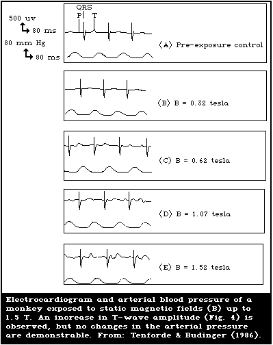 From the theoretical discussion in section 4, four predictions
can be made regarding the induced blood flow potential and the
associated magnetohydrodynamic effects:
(a) an induced flow potential should have a linear
dependence on the applied magnetic field strength;
(b) the magnitude of the potential should be a function
of the orientation of the animal relative to the
field direction;
(c) the induced potentials observed in the ECG should
increase with the size of the animal;
(d) the resultant magnetohydrodynamic effects should be
small.
In the following section, experimental data will be described
that relate to these predictions.
5.4.1. Linear relationship of induced flow potential and magnetic
field strength
Experimental tests of the linear relationship between the
magnetically-induced aortic blood flow potential and the applied
magnetic field strength have been carried out by recording the ECG
of several species of mammals during exposure to graded field
intensities. From the ECG records of rats exposed to static fields
ranging from 0.1 to 2.1 T, a field-strength-dependent increase in
T-wave amplitude was observed at field levels greater than 0.3 T
(Gaffey & Tenforde, 1981). The T-wave signal increase was a linear
function of the applied field up to 1.4 T. In dogs (Gaffey &
Tenforde, 1979), baboons (Gaffey et al., 1980), and monkeys
(Tenforde et al., 1983), the threshold for detection of the T-wave
amplitude change was 0.1 T, and the increase in signal strength was
a linear function of the magnetic field up to 1 T (Fig. 7).
These data support the concept that the T-wave alteration is a
consequence of the superposition of an induced aortic blood flow
potential, which is theoretically predicted to have a strictly
linear dependence on the magnetic field strength.
5.4.2. Induced flow potentials and field orientation
From theoretical considerations, it is predicted that the
magnitude and the sign of the induced flow potential should be a
function of the angle between the direction of blood flow and the
direction of the applied magnetic field. Consistent with this
prediction, it has been shown for rabbits (Togawa et al., 1967) and
for rats (Gaffey & Tenforde, 1981) that the amplitude of the T-wave
signal can be increased, decreased, or remain unchanged by the
superimposed aortic blood flow potential, depending on the
orientation of the animal relative to the field. It has also been
demonstrated that the maximum change in the T-wave amplitude occurs
when the long axis of a rat, and hence its ascending aortic vessel,
is oriented perpendicular to the field (Gaffey & Tenforde, 1981).
This observation is completely consistent with the theoretical
prediction that the magnitude of the magnetically-induced aortic
blood flow potential should achieve its maximum value when the flow
vector and the magnetic field vector are orthogonal.
5.4.3. Dependence of induced blood flow potentials on animal size
The theoretical considerations in section 4 suggest that the
magnitude of induced aortic blood flow potentials should be
significantly greater for large animal species than for the rodent.
When ECG measurements were made on animals exposed to a 1-T field,
with an orientation perpendicular to the body axis, the maximum
aortic flow potentials recorded at the body surface were 75 µV for
rats (average weight 0.25 kg) (Gaffey & Tenforde, 1981), 175 µV for
baboons (5 kg) (Gaffey et al., 1980), 200 µV for monkeys (5 kg)
(Tenforde et al., 1983), and 390 µV for dogs (9 kg) (Gaffey &
Tenforde, 1979). Thus, greater magnetically-induced blood flow
potentials were observed with larger animal species, conforming to
theoretical expectations.
5.4.4. Magnetohydrodynamic effects
A test of potential alterations in haemodynamic parameters as a
consequence of magnetohydrodynamic interactions was made by
recording the arterial blood pressure of monkeys during exposure to
homogeneous, static magnetic fields ranging from 0.1 to 1.5 T. The
study was conducted with an accuracy of ± 2 mmHg in the recording
of systolic and diastolic blood pressures. No measurable
alteration in blood pressure was observed in fields up to 1.5 T
(Fig. 7). This observation is consistent with the theoretical
prediction that negligible haemodynamic alterations result from
magnetohydrodynamic interactions with blood flow in fields of less
than 2 T (Tenforde et al., 1983).
5.4.5. Cardiac performance
Several indices of cardiac function have been studied in order
to assess the possible physiological effects of the electrical
potentials induced by an applied magnetic field. These indices
include blood pressure, heart rate, and the bioelectric activity of
heart muscle. As described above, there is no measurable
alteration in the blood pressure of monkeys exposed to a 1.5-T
stationary field. The heart rate and electrical properties of
heart muscles have been determined from ECG measurements on rats
exposed to stationary fields up to 2.1 T (Gaffey & Tenforde, 1981),
rabbits in a 1-T field (Togawa et al., 1967), dogs (Gaffey &
Tenforde, 1979) and baboons (Gaffey et al., 1980) in fields up to
1.5 T, and monkeys exposed to fields of up to 1.5 T (Tenforde et
al., 1983) and to a 10-T field (Beischer, 1969). Significant
changes in heart rate were not observed during acute magnetic field
exposures in any of these studies. Similarly, the amplitudes of
the P, Q, R, and S waves of the ECG were not altered, indicating
that the applied magnetic field had no effect on the depolarization
characteristics of the auricular and ventricular heart muscle. The
data from these studies on various species of animals also
indicated that no cardiac arrhythmias occurred during acute
exposures to the field levels studied.
These experimental observations provide evidence that little or
no cardiovascular stress should result from exposure to the highest
static magnetic field levels routinely encountered by man.
However, this conclusion must be tempered by the recognition that
no data are available in the literature relating to cardiovascular
performance during protracted exposure to large stationary magnetic
fields. Also, from the theoretical considerations discussed in
section 4, it would be anticipated that measurable haemodynamic
pertubations could occur during exposure to static fields that
significantly exceed 2 T. For example, it has been predicted
theoretically (Tenforde, 1985a) that a 5-T field would produce a
reduction in aortic blood flow velocity of up to 7% in a human
adult.
5.5. Nervous System and Behaviour
On the basis of the theoretical models described in section 4,
it is not anticipated that stationary magnetic fields with
intensities up to 2 T would produce measurable alterations in nerve
bioelectric properties. The theoretical expectations agree with
the existing experimental information on the behaviour of isolated
neurons in large static magnetic fields.
5.5.1. Excitation threshold of isolated neurons
From the theoretical considerations of Wikswo & Barach (1980),
it can be estimated that a static magnetic field of at least 24 T
would be needed to reduce the velocity of action potential
conduction in isolated neurons by 10%. The threshold for neural
excitation has been examined for both intact frog sciatic nerves
and single myelinated sciatic nerve fibres during exposure to a
homogeneous, static magnetic field (Liberman et al., 1959; Gaffey &
Tenforde, 1983). In both studies, the field orientation was
transverse to the nerve axis. No evidence was obtained in these
studies of an effect of a 1-T magnetic field on the minimum
electrical stimulus required to evoke action potentials in either
single fibres or intact sciatic nerves.
An important observation that has a direct bearing on such
studies was made by Gaffey & Tenforde (1983), who determined the
temperature coefficient of the frog sciatic nerve excitation
threshold, and found it to rise with increasing temperature. To
obtain reliable results, it was found that the temperature must be
controlled to within 0.1 °C.
5.5.2. Action potential amplitude and conduction velocity in
isolated neurons
Several groups of investigators have studied the properties of
evoked action potentials in isolated nerve preparations during
exposure to static magnetic fields oriented either parallel or
perpendicular to the nerve axis. Schwartz (1978) exposed the
circumoesophageal nerve of the lobster to static fields with a
maximum strength of 1.2 T. The nerve preparation was maintained in
an L-shaped chamber, and the field gradient along the sections of
nerve oriented parallel and perpendicular to the field lines were 2
and 15 T/m, respectively. No effects of either the parallel or
perpendicular fields, applied for periods of up to 30 min, were
observed on the nerve conduction velocity. Gaffey & Tenforde
(1983) conducted similar measurements on intact sciatic nerves
exposed to either parallel or perpendicular 2-T static fields that
were homogeneous to within 0.1% over the entire length of the
nerve. With both field configurations, no effects were observed
during a continuous 4-h exposure on either the amplitude or the
conduction velocity of maximal evoked action potentials. Extending
the duration of exposure to 17 h was also found not to influence on
the impulse conduction velocity.
Schwartz (1979) measured the membrane potentials and
transmembrane currents in lobster circumoesophageal nerves exposed
to a 1.2-T stationary field. Both parallel and perpendicular field
orientations relative to the nerve axis were used in these
experiments, and the field gradients were identical to those
described above in the discussion of Schwartz's studies on nerve
conduction velocity (Schwartz, 1978). No effects of the parallel
or perpendicular magnetic fields were observed on either the action
potentials or the transmembrane currents during nerve excitation.
In contrast to the negative results of the studies described
above, the results of two other studies have shown effects of
static magnetic fields on nerve bioelectric activity (Reno, 1969;
Edelman et al., 1979). However, Tenforde (1985b) suggested that
the apparent magnetic field effects observed in these studies are
probably attributable to a lack of precise temperature control, the
importance of which has already been discussed above.
5.5.3. Absolute and relative refractory periods of isolated neurons
Following the passage of a maximal action potential, an
isolated peripheral nerve enters an absolute refractory period of 1
- 2 ms duration, during which a second impulse cannot be evoked.
Following the absolute refractory period, the nerve enters a
relative refractory period during which action potentials of
progressively increasing amplitude can be evoked by electrical
stimulation. After a period of approximately 4 - 6 ms, the second
action potential reaches the same maximal amplitude as the impulse
elicited by the initial stimulus, thus marking the end of the
relative refractory period. The characteristics of both the
absolute and relative refractory periods have been examined during
the exposure of frog sciatic nerves to a homogeneous 2-T field
(Gaffey & Tenforde, 1983; Tenforde et al., 1985). Using both
parallel and perpendicular configurations of the magnetic field
relative to the nerve axis, no influence of the field was observed
on the duration of either the absolute or the relative refractory
periods. In addition, the amplitudes of impulses evoked during the
relative refractory period were unaffected by the magnetic field
exposure.
In summary, the majority of the experimental studies that have
been conducted to date indicate that static magnetic fields up to 2
T have little or no influence on the bioelectric properties of
isolated neurons.
5.5.4. Effects of static magnetic fields on the electroencephalogram
Several reports have been made of changes in brain electrical
activity during the exposure of experimental animals to static
fields ranging from approximately 0.1 to 9.1 T. The information is
inconsistent, at times contradictory, and requires additional
investigations before a definite judgement can be made.
In a series of electroencephalogram (EEG) studies on squirrel
monkeys, Beischer & Knepton (1966) observed that exposure to static
magnetic fields produced a significant increase in the amplitude
and frequency of brain electrical signals recorded below the scalp
in the frontal, parietal, temporal, occipital, and median cranial
regions. Recordings of the EEG were made in homogeneous fields
with field strengths ranging from 1.47 to 9.13 T. EEG recordings
were also made in strong gradient fields. During exposures ranging
from 3 to 45 min, it was found that the predominant EEG frequencies
shifted from their pre-exposure range of 8 - 12 Hz to 14 - 50 Hz,
independently of the field intensity or homogeneity. The
amplitude of the signals also increased from the control level of
25 - 50 µV to 50 - 400 µV. These changes were uniformly observed
in the different cranial regions, which were simultaneously
monitored; there was no latency in the response on application of
the field. When the field was removed, both the amplitude and
frequency spectrum of the EEG signals returned to their pre-
exposure levels, indicating the transient nature of this effect.
In analysing the results of their studies, Beischer & Knepton
(1966) considered several potential sources of artifacts,
including ripple currents from the magnet power supply, animal
movements associated with heart contractions and breathing, pick-up
of stray 60-Hz fields by the EEG electrodes and leads, and skeletal
muscle tremors. All of these factors, except for muscle tremors,
could be excluded because their characteristic frequencies were
outside the frequency range observed for the predominant EEG
signals in the presence of a static magnetic field. However, the
characteristics of the EEG tracings obtained from monkeys in the
magnetic field suggest that "myographic noise" from skeletal
muscles may have been superimposed on the brain electrical signals.
It is also possible that other uncontrolled factors, present only
during excitation of the magnet coils, including mechanical
vibrations, audible noise, and an increased ambient temperature,
could have led to an altered pattern of brain electrical activity.
In contrast to the above findings with monkeys, Kholodov
reported that the exposure of rabbits to relatively weak static
fields (0.08 - 0.10 T) produced an EEG signature characteristic of
a general inhibitory state in the central nervous system (Kholodov,
1964, 1966; Kholodov et al., 1969). The major changes in the EEG
during magnetic field exposure were the occurrence of slow waves
and high-amplitude spindles observed in the electrical activity
recorded from different regions of the brain. The phenomenon was
not uniformly exhibited in all of the tests conducted by Kholodov;
in a series of 100 field exposures on 12 rabbits, the author
observed the occurrence of spindles in 30% of the tests, and an
increase in the number of slow waves with frequencies of less than
4 Hz in 19% of the tests (Kholodov, 1966). The percentage of
animals exhibiting EEG responses to the field was not stated. Both
spindles and slow waves in the EEG occurred with a latency of
approximately 15 s after the field was turned on, and reached
maximum levels after 45 s of exposure. The increased number of
spindles and slow waves persisted during exposure to a 0.1-T field
for 3 min, and decreased immediately after the field was turned
off. However, 15 to 25 s after the exposure was terminated, a
transient increase in the number of spindles and slow waves
occurred with a duration of approximately 20 - 30 s.
Kholodov (1966) presented evidence that the EEG alterations
observed in his studies on rabbits were not artifacts resulting
from the induced potentials that occur during the switching on and
off of an electromagnet. This possibility was excluded on the
basis of trials in which the magnet was energized and de-energized
at various rates, with no resulting change in the character of the
observed EEG alterations.
Kholodov (1966, 1981, 1982) also described histological changes
in the brains of mammals exposed to static magnetic fields for
brief periods. The significance of these anatomical changes was not
clearly established. The differences in the results obtained by
Beischer & Knepton (1966) and by Kholodov (1966) may be related to
the one order of magnitude difference between the field strengths
used in their studies. Furthermore, Battocletti et al. (1981) did
not find changes in potentials evoked by stimulation of extremities
in rhesus monkeys exposed to 2 T for 48 h.
The positive observations may be explained by additive effects
on elements of the central nervous system (Valentinuzzi, 1965).
It should be noted that no recent studies on the effects of static
magnetic fields on the bioelectric activity of the brain were found
in the published literature. It seems that this area deserves
further study using modern electroencephalographic methods. The
application of recordings from single locations in the brain to
elucidate the neural basis for sensitivity to magnetic cues in
pigeons (Semm et al., 1984; Semm, 1986) may serve as an example.
5.5.5. Behavioural effects
An inherent sensitivity to the weak geomagnetic field and
correlated behavioural responses has been demonstrated for a number
of different organisms and animal species. It has been well
documented experimentally that weak magnetic fields influence the
migratory patterns of birds (Keeton, 1971; Emlen et al., 1976;
Bookman, 1977), the kinetic movement of molluscs (Ratner, 1976),
the waggle dance of bees (Martin & Lindauer, 1977), the direction-
finding of elasmobranch fish (Kalmijn, 1978, 1982), and the
orientation and swimming direction of magnetic bacteria (Blakemore,
1975; Blakemore et al., 1980). The mechanisms underlying the
magnetic sensitivity of elasmo-branchs and magnetotactic bacteria
have been discussed in sections 4.1.1 and 4.1.2.2.
A precise mechanism underlying the magnetic sensitivity of
other organisms has not been elucidated, although small deposits of
magnetite crystals have been discovered in the cranium of pigeons
(Walcott et al., 1979), in the tooth denticles of molluscs
(Lowenstam, 1962; Kirschvink & Lowenstam, 1979), and in the
abdominal region of bees (Gould et al., 1978). Magnetite has been
also reported in various anatomical sites in dolphins (Zoeger et
al., 1981), tuna (Walker et al., 1984), butterflies (Jones &
MacFadden 1982), turtles (Perry et al., 1981), mice (Mather &
Baker, 1981), and human beings (Kirschvink, 1981; Baker et al.,
1983). The possible role of magnetite in the geomagnetic
direction-finding mechanism possessed by some of these species has
not been established, nor is it clear for all of the mammalian
species in which magnetite deposits have been reported to occur
(Baker, 1980; Gould & Able, 1981).
Although the directional cues derived from the weak geomagnetic
field by certain species of animals have been demonstrated by
careful study, the possible effects of magnetic fields on the
behaviour of higher organisms are by no means established. Several
studies with rodents have reported effects of static magnetic
fields of less than 1 T on locomotor activity and patterns of food
and water consumption (Aminev et al., 1967; Russell & Hendrick,
1969; Pelyhe et al., 1973; Nakagawa, 1979; Nakagawa et al., 1980;
Shust et al., 1980). In contrast to these earlier reports, Davis
et al. (1984) did not observe any behavioural abnormalities in mice
exposed for prolonged periods to a 1.5-T field. The behavioural
end-points examined in this extensive study included memory
retention of an electroshock-motivated passive avoidance task,
general locomotor activity, and sensitivity of the subjects to a
neuropharmacological agent (pentylenetetrazole). Smirnova (1982)
also did not find any behavioural effects in rats exposed to 0.3 T
or 1.6 T for 5 min/day for 3 successive days.
The effects on primate behaviour of exposure to intense
magnetic fields was studied by Thach (1968). In one study, 3
squirrel monkeys (Saimiri sciureus) were conditioned to respond to
a visual vigilance task and subsequently exposed to static magnetic
fields in the core of a water-cooled Bitter magnet. Response was
greatly suppressed by fields of 7 T or more. A threshold seemed to
exist between 4.6 and 7 T. In a second study (deLorge, 1979), 8
squirrel monkeys were trained in several operant tasks and a
similar suppression response was observed in fields up to 9.7 T.
In addition, 2 of the monkeys regurgitated when exposed to these
higher fields. All of these effects were reported to be
reproducible.
5.6. Visual System
As discussed in section 4.2, one of the most clearly
established magnetic field effects in biological systems is the
phenomenon of magnetophosphenes, in which a flickering light is
produced in the visual field during exposure to time-varying
magnetic fields.
Although the phenomenon of phosphenes has not been reported by
human observers during exposure to large static magnetic fields,
there are two potential interaction mechanisms between these fields
and elements of the retina that are involved in the visual response
to photic stimulation. First, the photoreceptor outer segments
are subject to orientation in a static magnetic field as the result
of their large diamagnetic anisotropy (Chalazonitis et al., 1970;
Hong et al., 1971; Becker et al., 1978b; Hong, 1980). Second, the
initial photoisomerization event elicited by photon absorption in
retinal photopigments is followed by a series of ionic fluxes that
lead to excitation of the retinal neurons, and ultimately the
visual cortex via a complex neural pathway. This component of the
phototransduction process could be influenced by static magnetic
fields as the result of ionic current distortion and/or inductive
effects, as discussed in section 4. However, electrophysiological
studies on the retinal response to photic stimuli in cats and
monkeys have not shown any effects of exposure to a 1.5-T static
magnetic field (Gaffey & Tenforde, 1984; Tenforde et al., 1985).
That photoreceptors may play a crucial role in magneto-
reception is suggested by the fact that inhibitory effects of low
magnetic fields on pineal melatonin synthesis were not found in
albino rats (Olcese et al., 1985) or in rats exposed to magnetic
fields in total darkness (Reuss & Olcese, 1986), thus supporting
the theory of Leask (1978) that incident radiation is an important
factor in magnetic field sensitivity, i.e., light might be
essential to the process of magnetoreception. In contrast to rats
(both albino and pigmented strains), hamsters did not respond to
magnetic stimuli, as measured by the inhibition of pineal gland
metabolism (Olcese & Reuss, 1986), and species-specific differences
as well as reciprocal effects between photoreceptors and retinal
pigments should be taken into consideration.
Since birds possess a direction-finding sense that appears to
be based on simultaneous detection of the earth's magnetic and
gravitational fields, Semm et al. (1984) undertook a study to
explore possible neural mechanisms for the integration of magnetic
and gravitational cues. Leask (1977) proposed that the magnetic
field compass was located in the retina of the bird. Thus, Semm et
al. (1984) recorded single unit electrical activity in the lateral
and superior vestibular nuclei, the vestibulo-cerebellum, and the
nucleus of the basal optic root, which has a projection to the
vestibular system, in pigeons, under magnetic stimulation by fields
of about 42 µT. The responses of these cell systems were
direction-selective, i.e., different cells responded to different
directional changes in the magnetic field. The interpretation of
this was that magnetic cues may be conveyed from the visual to the
vestibular system via a projection from the basal optical root, and
then related to the movement of the bird.
The effects of static magnetic fields on turtle retinas in
vitro were studied by Raybourn (1983) (see also Tenforde et al.,
1985). No changes were seen in electroretinograms (ERG) from dark-
or light-adapted eyes during exposure to 1-T fields. However, 2-
to 3-mT fields suppressed the B-wave of the ERG in eyes prepared
during the light-to-dark adaptation phase, which lasts for about 2
h. No effects of 1.5-T fields on the ERG in cats and monkeys were
observed (Gaffey & Tenforde, 1984; Tenforde et al., 1985), but
circadian variations were not studied. These findings have not
been interpreted. The static magnetic field strength at which
effects were noted in turtle retinas was too low to influence ionic
fluxes that occurred in the retina following stimulation by light.
5.7. Physiological Regulation and Circadian Rhythms
In assessing the responses of living organisms to static
magnetic fields, an important aspect is the maintenance of normal
homeostatic regulation. The literature on this subject is often
contradictory. For example, the finding by Sperber et al. (1984)
that thermoregulation in rodents is affected by strong magnetic
field spatial gradients, could not be replicated by Tenforde
(1986c). It should be noted that Gremmel et al. (1984) described
changes in thermoregulation in human beings exposed to magnetic
fields. One of the central issues in this assessment is whether
exposure to magnetic fields produces an alteration in the normal
circadian rhythm of major physiological and behavioural variables.
Several of the investigations discussed in this section indicate
that exposure of mammals to static magnetic fields may lead to
hormonal alterations and to other metabolic effects that could
potentially affect physiological regulation, and thereby lead to an
alteration in the normal circadian rhythm. Although there is
relatively little information available on this subject, several
reports in the literature suggest that weak magnetic fields may
influence circadian regulation.
Brown & Scow (1978) observed a modulation of the normal 24-h
circadian activity period in hamsters, when a weak magnetic field
with a maximum intensity of 26 µT was applied in 26-h cycles. The
nocturnal sensitivity of mice to morphine was found by Kavaliers et
al. (1984) to be diminished, when the animals were exposed to a
rotating magnetic field with an intensity ranging from 105 µT to
9 mT. A cancellation of the earth's magnetic field by Helmholtz
coils was found to alter the circadian activity of birds (Bliss &
Hepner, 1976). It has recently been reported that artificial
changes in the strength and direction of the local geomagnetic
field are sufficient to alter the electrical activity of pineal
cells in the guinea-pig (Semm et al., 1980; Semm, 1983), rat (Reuss
et al., 1983), and pigeon (Semm et al., 1982, 1984; Semm, 1983,
1986). In related studies, it was demonstrated in albino rats that
artificial changes in the ambient magnetic field reduced the
nocturnal rise in pineal melatonin contents and the activity of the
involved enzymes, N -acetyltransferase (Welker et al., 1983; Olcese
et al., 1985; Olcese & Reuss, 1986) and hydroxyindole- O -
methyltransferase (Reuss & Olcese, 1986). Interestingly, this
effect was not found using NMR-strength fields of 0.14 T (Reuss et
al., 1985).
In other recent studies (Tenforde, 1985c; Tenforde et al.,
1986b,), prolonged exposures of mice to a 1.5-T static magnetic
field did not produce any alterations in the circadian rhythm of
several physiological and behavioural variables. Noninvasive
transducer techniques were used to provide continuous measurements
of core body temperature, respiration, body mass, food intake and
excreta, and two independent indices of locomotor activity. The
rodents were subjected to a homogeneous 1.5-T field under 3
different exposure regimens: (a) continuous exposure for 5 days;
(b) intermittent exposure in an 8 h-on/16 h-off cycle for 10
consecutive days; and (c) serial exposures to the field under the
5-day continuous and 10-day intermittent schedules. In addition,
the sensitivity of circadian oscillations to a 1.5-T field was
tested both in mice that were maintained on a diurnal light/dark
cycle, and in mice that were placed in a free-running circadian
state by the maintenance of continuous dim illumination. Under all
of these conditions, no influence of a 1.5-T field was observed on
the circadian variations in any of the physiological or behavioural
parameters studied.
In an effort to elucidate whether static magnetic fields
perturb the light-elicited electrical activity of the retina,
Raybourn (1983) recorded the external ERG of isolated turtle
retinas during light stimulation in the presence of magnetic fields
of graded strength. When the retinal preparations from light-
adapted or dark-adapted eyes were studied, no changes in the ERG
occurred in fields up to 1 T. However, the amplitude of the ERG
b-wave, which results from the electrical activity of nerve cells
in the retina, was consistently suppressed in retinas prepared
during the light-to-dark transition phase of the diurnal 12 h-
light/12 h-dark cycle. During this transition phase, which extended
for approximately 2 h after the onset of darkness, the
photoreceptor cells underwent rapid changes in both physiological
and metabolic activities (Bubenik et al., 1978; Young, 1978).
The magnetic field effect was observed with intensities as low
as 2 - 3 mT, and was rapidly reversible following termination of
exposure. This effect was observed in both the cone-dominant
retinas of Pseudemys scripts turtles, and the mixed rod-cone
retinas of Chelydra serpentina turtles, suggesting that it is
independent of the photoreceptor cell type. The circadian
dependence of the magnetic field sensitivity was clearly
demonstrated by studies in which the light/dark cycle was phase
shifted by several hours (Tenforde et al., 1985).
An alteration in human twilight visual acuity has been reported
to occur in response to changes in the strength of the ambient
geomagnetic field (Krause et al., 1984). It has been suggested
that this visual alteration may have its origin in a quantum
mechanical effect on biochemical reactions in the retina, similar
to that discussed by Schulten et al. (1978).
5.8. Genetics, Reproduction, and Development
Developing organisms frequently exhibit a strong response to
noxious environmental factors. This observation has stimulated a
relatively large number of studies on the potential effects of
static magnetic fields on the genetics, reproduction, and
development of various organisms. Investigations on a variety of
non-mammalian test systems have led to several reports of mutagenic
and developmental effects resulting from exposure to both gradient
and homogeneous magnetic fields. Effects observed with strong
magnetic field gradients have included alterations in the sex ratio
and development of Drosophila pupae (Mulay & Mulay, 1964; Markuze
et al., 1973; Tvildiani et al., 1981), and abnormal development of
sea urchin, frog, and salamander eggs (Perakis, 1947; Neurath,
1968; Levengood, 1969; Ueno et al., 1984). Inhibition of limb
regeneration in crabs (Lee & Weis, 1980) has also been observed.
Homogeneous magnetic fields have been reported to alter the
development of chicken embryos (Joshi et al., 1978), and guppies
(Brewer, 1979), and the rate of fertilization of trout eggs (Strand
et al., 1983). It is interesting to note that Perakis (1947) did
not find any effects of a homogeneous 3.3-T field on the
development of sea urchin eggs, and Ueno et al. (1984) did not
observe any effects of a 1-T homogeneous field on the development
of frog embryos. The absence of effects of homogeneous magnetic
fields on frog egg development is also supported by the
experimental observations of Iwasaki et al. (1978) and Mild et al.
(1981). In contrast, developmental abnormalities were observed in
both sea urchin eggs and frog embryos exposed to large magnetic
field gradients (Perakis, 1947; Ueno et al., 1984). Ueno et al.
(1984) suggested that the developmental effects of gradient fields
may result from a redistribution of dissolved oxygen or from the
orientation of mitochondrial cytochromes in large magnetic fields
with gradients exceeding 104 T/m.
In studies on mammals, it has been reported that homogeneous
and gradient fields up to 0.94 T inhibit weight gain in young mice
and produce weight loss in older animals (Barnothy, J.M., 1964).
The rate and number of live births and the average birth weight
have also been reported to decrease following prenatal and
postnatal exposure of mice to a homogeneous field (Nakagawa, 1979).
In contrast to these reports, studies on young mice exposed for up
to 15 days to a nearly homogeneous field with a maximum strength of
1.44 T did not reveal any effects on growth rate (Eiselein et al.,
1961). Bellossi et al. (1984) did not observe any variations in
growth of either mice or rats exposed to static magnetic fields of
up to 800 mT for up to 250 days. The intrauterine exposure of mice
and rats to either a 1-T homogeneous field or a 2.5-T/m gradient
field was also found not to influence fetal or postnatal
development (Sikov et al., 1979).
Exposure of mice to static magnetic fields of 1.6 T, during a
30-day period, resulted in reversible changes in spermatogenic
epithelium and in a considerable decrease in the number of mature
germ cells (Galaktionova et al., 1985). These and other authors
(Toroptsev et al., 1974; Udintsev & Khlynin, 1979) considered the
testes a vulnerable organ when exposed to static or time-varying
(20 mT, 50 Hz) magnetic fields. Morphological changes in the
testes and other organs, which occur after a 6-h exposure to
magnetic fields, revert to normal after approximately one month.
Several studies have been carried out to determine whether
genetic defects can be detected following magnetic field exposure.
No increase in mutation frequency was observed by Kale & Baum
(1979) among the progeny of Drosophila males exposed as eggs,
larvae, pupae, and adults to 1.3 - 3.7-T homogeneous magnetic
fields. Similar results were obtained by Mittler (1971) and
Diebolt (1978), who exposed Drosophila males to fields of 1 -
1.1 T. Baum et al. (1979) also found that exposure of the plant
Tradescantia to homogeneous fields up to 3.7 T did not lead to any
increase compared with controls in three mutagenic indices, namely,
pollen abortion, micronuclei formation, and pink stamen hair
production. Dominant lethal assays have been conducted by Mahlum et
al. (1979) with male mice exposed to either a uniform 1-T or a 2.5-
T/m gradient field for 28 days prior to mating. No effects of
exposure to either the homogeneous or the gradient field were
observed. This result and the study of Strzhizhovsky et al.
(1980) indicate that such exposure does not induce chromosomal
aberrations in male germ cells.
Recent studies have also demonstrated that the exposure of
cultured Chinese hamster ovary cells to a 0.35-T homogeneous field
does not lead to alteration in DNA synthesis or chromosome
structure (Wolff et al., 1980). The structure and biological
activity of bacteriophage DNA have also been found to be unaffected
by exposure to a 2-T homogeneous field (Roots et al., 1982).
5.9. Conclusions
Studies on the effects of static magnetic fields on enzyme
reactions and cellular and tissue functions have provided diverse,
and often contradictory, findings. Nevertheless, available
evidence indicates that there are few irreversible effects on such
systems, with the possible exception of:
(a) enzymes and photosynthetic systems that involve
radical-mediated reaction intermediates; and
(b) cellular systems in which the membrane is undergoing
a structural phase transition during magnetic field
exposure.
The occurrence of significant genetic or developmental
alterations in cellular tissues and animal systems exposed to high-
intensity static magnetic fields appears unlikely from available
evidence. One possible exception relates to unconfirmed reports of
alterations in the embryonic development of amphibian species
exposed to strong magnetic field gradients.
The magnetic induction of electrical potentials and currents in
the central circulatory system does not produce measurable
cardiovascular stress during short-term exposure to static fields
of up to 2 T. This conclusion must be tempered by the recognition
that data do not exist on cardiovascular performance during
protracted magnetic field exposure.
The majority of experimental studies conducted with isolated
neurons indicate that static magnetic fields of up to 2 T have no
irreversible influence on neuronal bioelectric properties. Several
reports have referred to changes in brain electrical activity and
behaviour in animals exposed to fields ranging from 0.1 to 9 T, but
the data are inconsistent and at times contradictory.
An inherent sensitivity to the weak geomagnetic field and
correlated behavioural responses have been demonstrated for a
number of different organisms and animal species. However,
behavioural effects in higher organisms have not been established
at field strengths of less than 2 T. Although the data are
inconsistent, effects on physiological regulation and circadian
rhythms have been reported in animals, due to alterations in the
local geomagnetic field. Negative findings in higher organisms
have been reported in studies involving field levels as high as
1.5 T.
Thus, reversible or transient effects have been reported in
lower animals due to exposure to low-intensity static fields or due
to alterations in the ambient geomagnetic field. However, no
irreversible effects have been established due to static magnetic
field exposures of up to 2 T.
6. BIOLOGICAL EFFECTS OF TIME-VARYING MAGNETIC FIELDS
An extensive literature exists on the response of animals and
isolated cellular and tissue systems to ELF magnetic fields. At
present, this body of research is difficult to interpret in a
systematic manner because of two factors:
(a) A wide range of intensities, frequencies, waveforms, and
exposure durations have been used. Many of the earlier
studies involved sinusoidal fields oscillating at
frequencies below 100 Hz, but research during the last
several years has focused increasingly on the biological
effects of square-wave or pulsed fields with complex
waveforms.
(b) Very few of the reported effects of ELF magnetic fields
have been independently replicated in different
laboratories.
In spite of these difficulties, there is a growing body of
evidence that suggests that living systems exhibit a response to
ELF magnetic fields under conditions in which the field intensity
and rate of change in time (dB/dt) are sufficient to induce
currents greater than the naturally occurring levels in tissues and
extracellular fluids. This effect is best illustrated by the
phenomenon of magnetophosphenes, which is the one well established
biological effect of ELF magnetic fields. Although less well
established, there is also evidence suggesting that pulsed magnetic
fields, such as those used clinically to facilitate bone fracture
reunion, may exert direct biological effects through the induction
of tissue currents that exceed the endogenous levels.
The following topics are summarized in this section:
(a) magnetophosphene research;
(b) studies on the nervous system and animal behaviour;
(c) cellular, tissue, and animal responses to magnetic
fields with various waveforms and repetition
frequencies in the ELF range;
(d) studies on the effects of pulsed magnetic fields on
bone growth and repair; and
(e) thresholds for biological effects as a function of
field frequency and induced current densities.
6.1. Visual System
High-intensity magnetic fields oscillating in the ELF range
produce visual sensations in human subjects that are known as
magnetophosphenes. This phenomenon has already been discussed in
section 4.2.
Studies (Silny, 1981, 1984, 1986) have been performed to
characterize ELF magnetic-field effects on visually evoked
potentials (VEP). Fields greater than 50 mT in the frequency range
below 100 Hz were demonstrated to reverse the polarity and reduce
the amplitude of VEP recorded from human volunteers. This effect
persisted after the termination of the magnetic field exposure.
Approximately 40 min after the magnetic field exposure, the VEP was
found to return to a normal form. This effect of magnetic fields
was shown to be frequency-dependent, the field strength required to
elicit an alteration in the VEP decreasing as the field frequency
increased from 5 to 100 Hz. It should be noted that the field
strength required to alter the VEP is approximately one order of
magnitude greater than that required to elicit clear
magnetophosphene patterns.
6.2. Studies on Nerve and Muscle Tissue
Several studies have been made on the electrical response of
neurons to stimulation with time-varying magnetic fields. As
discussed by Bernhardt (1979, 1985), the current densities induced
by the field must exceed 1 - 10 mA/m2 in order to have an
appreciable effect on the nerve bioelectric activity, and a
threshold extracellular current density of about 20 mA/m2 has been
found experimentally with Aplysia pacemaker neurons stimulated
by an ELF electric field (Wachtel, 1979). In a subsequent study
with Aplysia (Sheppard, 1983), an induced current density of
approximately 5 mA/m2 produced by a 10-mT, 60-Hz sinusoidal field
was ineffective in altering the spontaneous neuronal electrical
activity. Ueno et al. (1981) were also unable to alter the
amplitude, conduction velocity, or refractory period of evoked
action potentials in lobster giant axons, by applying sinusoidal
magnetic fields with intensities of 1.2 T at 5 - 20 Hz, 0.8 T at 50
Hz, and 0.5 T at 100 Hz.
Using magnetic flux densities in the range of 0.2 - 0.8 T,
Kolin et al. (1959) were able to stimulate frog nerve-muscle
preparations at field frequencies of 60 and 100 Hz. Oberg (1973)
and Ueno et al. (1978) were also able to stimulate contractions in
frog nerve-muscle preparations by using pulsed magnetic fields with
pulse durations of less than 1 ms. In addition, the excitation of
frog sartorius and cardiac muscles (Irwin et al., 1970) and of the
sciatic nerves of dogs and rabbits (Maass & Asa, 1970) has been
reported to occur in response to pulsed magnetic fields. On the
basis of electromyographic recordings from the human arm, Polson
et al. (1982) were able to characterize the pulsed magnetic field
parameters that elicited a neural response. They indicated that
the threshold rate of change of the magnetic field (dB/dt), which
was necessary to stimulate the major nerve trunks of the arm, was
approximately 104 T/s. These fields were discrete pulses, 180 µs
long, which will result in a high threshold compared with that for
a continuously applied sinusoidal stimulus of between 10 and 100
Hz.
A threshold of perception of about 2 x 10³ T/s was reported
(McRobbie & Foster, 1984) in human volunteers whose forearms were
exposed to a damped sinusoidal magnetic field (2 - 3 cycles of a
period equal to 0.3 ms). The currents induced in the peripheral
tissues of the forearm were calculated to be approximately 5 A/m2.
Other effects of time-varying magnetic fields on electrically
excitable tissue have been summarized by Bernhardt (1985) (section
4.2). The frequency dependence of these effects has been described
by Bernhardt (1985, 1986) (section 8.2).
From these studies, it appears that sinusoidal magnetic fields
with intensities in the range generally used in the laboratory or
well above the levels encountered by human beings in occupational
settings or in the home environment, are insufficient to alter the
bioelectric properties of isolated neurons. However, direct
magnetic stimulation of nerve and muscle tissues can be achieved by
using pulsed fields with a rapid time rate of change of the
magnetic flux density. It should also be borne in mind that the
effects of sinusoidal fields on complex, integrated neuronal
networks, such as those within the central nervous system, may be
considerably greater than the effects that occur in single neurons
or nerve bundles. This amplification of a field effect could occur
through a summation of the small responses evoked in individual
neuronal elements (Valentinuzzi, 1965). An additive response
mechanism may also underlie the production of magnetophosphenes
through the stimulation of multiple neuronal elements of the retina
(Valentinuzzi, 1962).
6.3. Animal Behaviour
During the past two decades, a large number of studies on
animal behavioural responses to ELF magnetic fields have been
reported. A chronological listing of these reports and a summary
of the principal findings are given in Table 9.
Several studies in which the behaviour of honeybees and birds
was observed to be altered in the presence of combined ELF electric
and magnetic fields (Southern, 1975; Larkin & Sutherland, 1977;
Greenberg et al., 1981a,b) have not been included, because of
difficulty in attributing these effects to either the electric or
magnetic field component. In the case of bees, it appears that ELF
electric fields may induce step-potential currents in the hive that
have harmful effects when the field intensity exceeds approximately
2 kV/m (Greenberg et al., 1981b). However, altered behavioural
patterns in honeybees have also been reported to occur in strong
60-Hz magnetic fields in the absence of an external electric field
(Caldwell & Russo, 1968). The mechanism underlying the observed
disruption of avian migration by the 72- to 80-Hz electric and
magnetic fields from an ELF communication test system is not known
(Southern, 1975; Larkin & Sutherland, 1977). However, there are
numerous reports that weak static magnetic fields, comparable in
strength to the earth's field, may influence the migration patterns
of birds (Keeton, 1971; Emlen et al., 1976; Bookman, 1977) and very
weak time-varying magnetic fields have also been claimed to affect
avian orientation (Papi et al., 1983).
Table 9. Behavioural effects of exposure to time-varying magnetic fields
---------------------------------------------------------------------------------------------------------
Reference Subject Exposure conditionsa Results
---------------------------------------------------------------------------------------------------------
Friedman et al. human 0.1 and 0.2 Hz, 0.5 - 1.1 mT; Increased reaction time in 0.2-Hz field
(1967) being acute exposures
Caldwell & Russo honey 60 Hz, 2.2 - 30 mT; Altered exploratory behaviour
(1968) bee 10-min exposures
Persinger rat 0.5 Hz, 0.3 - 3 mT; rotating Decreased open-field activity and
(1969) field; exposure during entire increased defecation when tested
gestational period postnatally at 21 - 25 days
Persinger & Foster rat 0.5 Hz, 0.3 - 3 mT; rotating Decreased avoidance of aversive
(1970) field; exposure during entire electrical shock when tested
gestational period postnatally at 30 days
Grissett & deLorge monkey 45 and 75 Hz, 0.3 mT; fields No effect on reaction time
(1971) applied in 10 daily sessions
of 1 h duration
Grissett monkey 45 Hz, 1 mT; continuous No effect on reaction time
(1971) exposure for 42 days
Persinger & Pear rat 0.5 Hz, 0.3 - 3 mT, rotating Suppressed rate of response to a
(1972) field; exposure during entire conditioned stimulus preceding an
gestational period aversive shock when tested postnatally
at 70 days
Persinger et al. rat 0.5 Hz, 0.3 - 3 mT, rotating Increased ambulatory activity after
(1972) field; exposure of adult removal from field
animals for 21 - 30 days
Ossenkopp & Shapiro duck 0.5 Hz, 2 - 10 and 10 - 30 mT, Increased ambulation and defecation
(1972) egg rotating field; exposure for rate when tested postnatally
entire prenatal period
---------------------------------------------------------------------------------------------------------
Table 9. (contd.)
---------------------------------------------------------------------------------------------------------
Reference Subject Exposure conditionsa Results
---------------------------------------------------------------------------------------------------------
deLorge monkey 10, 15, 45, 60, and 75 Hz, No consistent influence on motor
(1972, 1973a,b, 0.8 - 1 mT; fields applied activity, reaction time, inter-response
1974, 1979, 1985) in 4 - 13 daily sessions of time, overall level responding, or
2- to 8-h duration match-to-sample performance
Beischer et al. human 45 Hz, 0.1 mT; 22.5-h exposure No effect on reaction time
(1973) being
Gibson & Moroney human 45 Hz, 0.1 mT; 24-h exposure No consistent effect on cognitive or
(1974) being psychomotor functions
Mantell human 50 Hz, 0.3 mT; 3-h exposure No effect on reaction time
(1975) being
Medvedev et al. human 50 Hz, 10 - 13 µT; acute Increased latency of sensorimotor
(1976) being exposures reactions
Smith & Justesen mouse 60 Hz, 1.4 - 2 mT; 2-min Increased locomotor activity and
(1977) aperiodic exposures over aggression-related vocalization
2 days
Andrianova mouse 100 Hz, 10 mT; acute exposures Heightened motor activity
& Smirnova
(1977)
Brown & Scow hamster 10-5 Hz, 0.8 - 26 µT; 26-h Modified circadian rhythm in locomotor
(1978) schedule of high (14 h) to activity
low (12 h) field switching
over period of 4 - 5 months
Tucker & Schmitt human 60 Hz, 1.06 mT over whole body, No perception of field
(1978) being or 2.12 mT over head region;
repetitive acute exposures
Becker, von termite 50 Hz, 0.05 µT in shielded room; Stimulation of gallery building
(1979) exposures up to several weeks activity
---------------------------------------------------------------------------------------------------------
Table 9. (contd.)
---------------------------------------------------------------------------------------------------------
Reference Subject Exposure conditionsa Results
---------------------------------------------------------------------------------------------------------
Clarke & Justesen chicken 60 Hz, 2.4 mT; aperiodic Increased variability of response to
(1979) exposures during 1-h interval electric shock stimulus when 60-Hz
for 10 days magnetic field used as conditional
stimulus
Udintsev & Moroz Rat 50 Hz, 20 mT, 15 min/day for Transitory stimulation of adrenal
(1982) 7 days system
Udintsev & Moroz rat 50 Hz, 20 mT, 6.5 h/day for Significant changes in hormone levels
(1982) 7 days
Delgado et al. monkey 9 - 500 Hz, 0.1 mT (applied Modification of threshold for
(1983) to cerebellum); 9-h daily exictation of motor neurons
exposures for maximum of
19 days
Papi et al. pigeon 0.034, 0.043, and 0.067 Hz, Initial disturbance of orientation, but
(1983) 60 µT peak intensity; no effect on homing performance
exposures up to 4 h
Graham et al. human 60 Hz, 40 µT; acute exposures No perception of field
(1984) being
Creim et al. rat 60 Hz; 3.03 mT; 1-h exposure No field-associated avoidance behaviour
(1984)
Davis et al. mouse 60 Hz; 2.33 mT; 3-day No change in memory retention,
(1984) continuous exposure locomotoractivity, or sensitivity to a
neuropharmacological agent
Liboff et al. rat 60 Hz, 56 µT (with a trans- Changes in timing discrimination
(1985) verse 26-µT static field);
30-min exposures
Creim et al. rat 60 Hz, 3 mT, 1- to 23-h No avoidance of applied field
(1985) exposures in a shuttle box test
---------------------------------------------------------------------------------------------------------
a The magnetic fields were sinusoidal unless otherwise indicated.
In assessing the effects of time-varying magnetic fields on the
behaviour of mammalian species, the publications on this subject,
listed in Table 9, are nearly equally divided between positive
findings and observations of no behavioural effects in mammals.
However, a careful examination of this list leads to the
interesting conclusion that most investigations in which
behavioural effects were not observed, the time rate of change of
the applied magnetic field was sufficient to induce peak
intracranial current densities at, or above, the endogenous level
of approximately 1 mA/m2. In contrast, only one of the positive
findings of behavioural alterations in mammals (Andrianova &
Smirnova, 1977) involved the use of a time-varying magnetic field
capable of inducing intracranial currents at this level.
In examining the possible reasons for this apparent disparity,
it is important to assess the potential influence on animal
behaviour of extraneous factors, such as mechanical vibration and
audible noise, that may accompany the activation of magnet coils.
The importance of these factors has been well demonstrated by
Tucker & Schmitt (1978), who found that perceptive individuals
could sense the presence of a 60-Hz magnetic field through
auxiliary clues. When these investigators developed an exposure
chamber that provided extreme isolation from vibration and audible
noise, none of the more than 200 individuals tested could detect
60-Hz fields with intensities of 1.1 mT over the whole body or 2.1
mT over the head region. The sensitivity of behavioural indices to
adventitious factors, such as changes in barometric pressure, was
also discussed by deLorge (1973b), who emphasized that the
correlation of such variables to positive findings of apparent
time-varying magnetic field effects must be examined.
6.4. Cellular, Tissue, and Whole Organism Responses
Magnetic fields with a broad range of intensities, ELF
frequencies, waveforms, and exposure durations have been evaluated
for their ability to induce effects at the cellular, tissue, and
animal levels. These studies have recently been reviewed
(Tenforde, 1985c, 1986a,d), and only a brief summary will be given
here of the cellular and tissue responses to ELF magnetic fields
that have been reported on the basis of both in vitro and in vivo
studies.
Reports of alterations produced in cellular, tissue, and animal
systems as a result of exposure to low frequency magnetic fields
are summarized in Table 10, where a brief summary is given of the
principal findings in each study. The following types of
investigations have not been included in Table 10 for the reasons
stated below:
(a) Studies on time-varying magnetic field effects on the
visual system (magnetophosphene induction), nervous
tissues, and animal behaviour, and epidemiological studies
on carcinogenic risk, because these subjects are discussed
elsewhere in this section and in section 8;
(b) Reports lacking adequate documentation of field
exposure conditions (e.g., frequency, waveform, intensity,
and duration of exposure). Similarly, studies in which
the biological measurements were qualitative rather than
quantitative, as in certain medical reports on bone
fracture reunion following therapy with pulsed magnetic
fields;
(c) Reports of research that involved combined exposures
to ELF electric and magnetic fields, because of the
obvious difficulty in delineating the relative effects of
the two types of fields.
The reported changes resulting from ELF magnetic field exposure
include the following:
(a) Altered cell growth rate (Batkin & Tabrah, 1977;
Tabrah et al., 1978; Goodman et al., 1979; Greenebaum
et al., 1979, 1982; Aarholt et al., 1981; Ramon et
al., 1981; Phillips et al., 1986a);
(b) Decreased rate of cellular respiration (Cook et al.
1969; Goodman et al., 1979; Greenebaum et al., 1979,
1982; Kolodub & Chernysheva, 1980);
(c) Altered metabolism of carbohydrates, proteins, and
nucleic acids (Udintsev et al., 1976, 1978; Kartashev
et al., 1978; Udintsev & Khlynin, 1979; Kolodub &
Chernysheva, 1980; Kolodub et al., 1981; Norton,
1982; Archer & Ratcliffe, 1983; Buyavikh, 1984;
Liboff et al., 1984);
(d) Effects on gene expression and genetic regulation of
cell function (Chiabrera et al., 1978, 1979; Beltrame
et al., 1980; Aarholt et al., 1982; Goodman et al.,
1983; Goodman & Henderson, 1986);
(e) Endocrine alterations (Riesen et al., 1971; Udintsev
& Moroz, 1974; Sakharova et al., 1977, 1981; Kolesova
et al., 1978; Udintsev et al., 1978);
(f) Altered hormonal responses of cells and tissues,
including effects on cell surface receptors (Dixey &
Rein, 1982; Luben et al., 1982; Marsakova, 1983;
Jolley et al., 1983; Cain et al., 1984; Chan &
Nicholson, 1986);
(g) Altered immune response to antigens and mitogens
(Odintsov, 1965; Mizushima et al., 1975; Conti et
al., 1983; Budd & Czerski, 1985);
(h) Morphological and other nonspecific tissue changes in
adult animals, frequently reversible with time after
exposure (Druz & Madiyevskii, 1966; Toroptsev et al.,
1974; Sakharova et al., 1981; Toroptsev & Soldatova,
1981; Soldatova, 1982; Shober et al., 1982);
(i) Teratological and developmental effects (Ossenkopp et
al., 1972; Delgado et al., 1981, 1982; Kreuger et
al., 1972; Ramirez et al., 1983; Ubeda et al., 1983).
Table 10. Effects of exposure to time-varying magnetic fields on cells, tissues, and whole animals
--------------------------------------------------------------------------------------------------------
Reference Test Exposure conditionsa Results
specimen
--------------------------------------------------------------------------------------------------------
Odintsov (1965) mouse 50 Hz, 20 mT; 6.5-h single Increased resistance to Listeria
exposure or 6.5 h daily for infection
15 days
Druz & Madiyevskii rat 3 Hz, 0.1 - 0.8 T, and 50 Hz, Change in hydration capacity
(1966) 0.05 - 0.2 T; 1-min exposures of brain, kidney, and liver tissues
Riesen et al. guinea-pig 60 Hz, 10 mT; 10 - 110-min No effect on respiration
(1971) brain exposures (oxidative phosphorylation)
mitochondria
in vitro
Riesen et al. rat brain 60 Hz, 5 - 10 mT; 30-min Decreased uptake of norepinephrine
(1971) synaptosomes exposure at 0 °C, but not at 10 °C, 25 °C,
in vitro or 37 °C
Tarakhovsky et al. rat 50 Hz, 13 - 14 mT; exposure Changes in serum chemistry,
(1971) for 1 month haematocrit, and tissue morphology
Kreuger et al. chicken 45 Hz, 0.14 mT, and 60 Hz, Reduced growth rate in young animals
(1972) 0.12-mT exposure for 1 month
Ossenkopp et al. rat 0.5 Hz, 0.05 - 0.30 or Increased thyroid and testicle weights
(1972) 0.3 - 1.5 mT, rotating field; at 105 - 130 days of age; no change in
exposure during entire thymus or adrenal weights compared
gestational period with controls
Beischer et al. human being 45 Hz, 0.1 mT; 22.5-h Elevated serum-triglycerides; no
(1973) exposure effects on blood cell counts or other
serum chemistry
DeLorge (1974) monkey 15 and 45 Hz, 0.82 - 0.93 mT; No alteration in blood cell counts or
fields applied in 5 - 8 daily serum chemistry (including trigycer-
sessions of 2-h duration ides)
--------------------------------------------------------------------------------------------------------
Table 10. (contd.)
--------------------------------------------------------------------------------------------------------
Reference Test Exposure conditionsa Results
specimen
--------------------------------------------------------------------------------------------------------
Toroptsev et al. guinea-pig 50 Hz, 20 mT; 6.5-h single Pathomorphological changes in testes,
(1974) exposure or 6.5 h daily for kidneys, liver, lungs, nervous tissues,
24 days eyes, capillaries, and lymphatic system
Udinstev & Moroz rat 50 Hz, 20 mT; 1 - 7 days Increase in adrenal 11-hydroxy
(1974) exposure corticosteroids
Mizushima et al. rat 50 Hz, 0.12 T; 3-h exposure Anti-inflammatory effects of field on
(1975) carrageenan-induced oedema and
adjuvant-induced arthritis
Beischer & Brehl mouse 45 Hz, 0.1 mT; 24-h exposure No change in liver-triglycerides
(1975)
Mantell (1975) human being 50 Hz, 0.3 mT; 3-h exposure No haematological changes
Udintsev et al. rat 50 Hz, 20 mT; 1-day Increased lactate dehydrogenase
(1976) exposure activity and change in distribution in
heart and skeletal muscles
Batkin & Tabrah mouse 60 Hz, 1.2 mT; 13-day Decreased tumour growth rate
(1977) neuroblastoma exposure
Sakharova et al. rat 50 Hz, 20 mT; 1-day Increased catecholamines in tissue
(1977) exposure
Kartashev et al. yeast 0.1 - 100 Hz, 0.025 - 0.40 Changes in rate of anaerobic glycolysis
(1978) mT; 20 - 30-min exposure
Kolesova et al. rat 50 Hz, 20 mT; single 24-h Development of insulin deficiency
(1978) exposure and 6.5 h daily
for 5 days
Tabrah et al. Tetrahymena 60 Hz, 5 - 10 mT; Cell division delay, reduced growth
(1978) pyriformis exposures up to 72 h rate, increased oxygen uptake
--------------------------------------------------------------------------------------------------------
Table 10. (contd.)
--------------------------------------------------------------------------------------------------------
Reference Test Exposure conditionsa Results
specimen
--------------------------------------------------------------------------------------------------------
Persinger et al. rat 0.5 Hz, 0.1 T - 1 mT, No significant changes in thyroid
(1978) rotating field; follicle numbers, mast cells, adrenal
10-day exposure and pituitary weights, body weight, or
water consumption
Persinger & rat 0.5 Hz, 0.01 T - 1 mT, No significant change in thymus mast
Coderre rotating field; 5-day cell numbers in animals exposed
(1978) exposure prenatally and postnatally or exposed
as adults
Udintsev et al. rat 50 Hz, 20 mT; 0.25- to Changes in iodine uptake by the thyroid
(1978) 6.5-h and 24 h exposures and thyroxine uptake by tissues
Udintsev & rat 50 Hz, 20 mT; 1-day Metabolic changes in testicle tissue
Khlynin (1979) exposure
Kronenberg & cultured 60 Hz, 2.33 mT; 4-day No effect on cell growth rate
Tenforde mouse exposure
(1979) tumour cells
Chandra & Stefani mouse 60 Hz, 0.16 T; 1-h daily No effect on tumour growth rate
(1979) mammary exposures for 1 - 4 days
carcinoma
Goodman et al. slime mould 75 Hz, 0.2 mT; 400-day Lengthened nuclear division cycle and
(1979); exposure altered respiration rate (decreased O2
Greenebaum et al. uptake)
(1979, 1982)
Chiabrera et al. frog Single bidirectional pulses Changes in chromatin structure in the
(1979) erythrocytes at 40 - 70 Hz, or 4-kHz bursts cell nucleus, suggestive of
of bidirectional pulses with dedifferentiation
10 - 20 Hz repetition rate;
2-mT peak intensity; 12- to
24-h exposures
--------------------------------------------------------------------------------------------------------
Table 10. (contd.)
--------------------------------------------------------------------------------------------------------
Reference Test Exposure conditionsa Results
specimen
--------------------------------------------------------------------------------------------------------
Kolodub & rat 50 Hz, 9.4, and 40 mT; Altered brain metabolism at higher
Chernysheva 5 h daily for 15 days field intensity, including decreased
(1980) rate of respiration, decreased levels
of glycogen, creatine phosphate and
glutamine, and increased DNA content
Fam (1981) mouse 60 Hz, 0.11 T; 23 h daily for Decreased body weight and increased
7 days water consumption; haematology, organ
histology and reproduction not affected
Aarholt et al. bacteria 16.66 and 50 Hz, 0 - 2 mT; Decreased growth rate
(1981) 10- to 12-h exposure
Ramon et al. bacteria 60 and 600 Hz, 2 mT; 17- to Decreased growth rate and cytolysis
(1981) 64-h exposure
Toroptsev & rat 50 Hz, 20 mT; 1- to 24-h Pathomorphological changes in brain
Soldatova exposure
(1981)
Kolodub et al. rat 50 Hz, 9.4 - 40 mT, daily Changes in carbohydrate metabolism
(1981) 3-h exposures for up to 6 in the myocardium
months
Sakharova et al. rat 50 Hz, 20 mT, 1-day exposure Changes in catecholamine content and
(1981) morphology in brain, heart, liver,
spleen, and circulatory system
Delgado et al. chicken 10, 100, and 1000 Hz; 0.12, Morphological abnormalities in nervous
(1981, 1982) embryo 1.2, and 12 µT; 0.5-ms tissue, heart, blood vessels, and
rectangular pulses; 2-day somites
exposure
Soldatova rat 50 Hz; 20, 40, and 70 mT; Pathomorphological changes in brain
(1982) 6.5 h daily for 5 days, or tissue
24-h continuous exposure
--------------------------------------------------------------------------------------------------------
Table 10. (contd.)
--------------------------------------------------------------------------------------------------------
Reference Test Exposure conditionsa Results
specimen
--------------------------------------------------------------------------------------------------------
Sander et al. human being 50 Hz, 5 mT; 4-h exposure No changes in ECG, EEG, hormones, blood
(1982) cell counts, or blood chemistry
Luben et al. mouse Single bidirectional pulses Reduced cAMP production in response
(1982) osteoblast at 72 Hz, or 4-kHz bursts of to parathyroid hormone
culture bidirectional pulses with
15 Hz repetition rate; 2 mT
peak intensity; 3-day exposure
Shober et al. mouse 10 Hz, 1 mT; 1-day exposure Decreased sodium ion content of liver
(1982)
Norton (1982) cultured 4 kHz bursts of bidirectional Increased hydroxyproline,
chicken pulses with 15 Hz repetition hyaluronate, and DNA synthesis;
embryo rate; 2 mT peak intensity; decreased glycosoaminoglycans;
sternum four 6-h exposures during 2 increased lysozyme activity
days
Aarholt et al. bacteria Square wave pulses at 50 Hz; Changes in rate of
(1982) (E. coli) 0.20 - 0.66 mT, 2- to 3-h beta-galactosidase synthesis
exposures
Dixey & Rein rat pheo- 500 Hz; bidirectional pulses; Stimulation of noradrenaline release
(1982) chromocytoma 160 - 850 µT; 3-h exposure
cell in
vitro
Conti et al. cultured 1, 3, 50, and 200 Hz; 2.3 - Inhibition of lectin-induced
(1983) human 6.5 mT; square-wave pulses; mitogenesis by 3- and 50-Hz fields
lymphocyte 3-day exposure
Goodman et al. sciara- Single bidirectional pulses Initiation and increase of RNA
(1983) coprophila at 72 Hz, or 4-kHz bursts of transcription at defined loci
salivary bidirectional pulses with 15
giant Hz repetition rate; 2 mT peak
chromosome intensity; 5- to 90-min
exposures
---------------------------------------------------------------------------------------------------------
Table 10. (contd.)
---------------------------------------------------------------------------------------------------------
Reference Test Exposure conditionsa Results
specimen
---------------------------------------------------------------------------------------------------------
Jolley et al. rabbit 4 kHz bursts of bidirectional Reduced Ca++ content and efflux;
(1983) pancreas pulses with 15-Hz repetition reduced insulin release during
rate; 2-mT peak intensity; glucose stimulation
18-h exposure
Ramirez et al. Drosophila 0.5-ms square-wave pulses at Decreased viability of eggs
(1983) egg 100 Hz, 1.76 mT peak-to-peak
intensity; or 50 Hz, 1.41 mT
sinusoidal field; 2-day
exposure
Ubeda et al. chicken 0.5 ms bidirectional pulses Teratogenic changes in nervous system,
(1983) embryo at 100 Hz (4 different circulatory system, and foregut
waveforms); 0.4- to 104-µT
peak intensity; 2-day
exposure
Archer & cultured 1 Hz, 15 - 60 mT square- Decreased collagenous and non-
Ratcliffe chicken wave pulses; 7-day exposure collagenous protein synthesis; no
(1983) tibia alteration in glycosoaminoglycan DNA
synthesis
Liboff et al. cultured 15 Hz - 4 kHz; 2.3 - 560 µT; Increased DNA synthesis
(1984) human 18- to 96-h exposures
fibroblast
Cain et al. cultured Single bidirectional pulses Inhibition of cAMP production and
(1984) mouse at 72 Hz, or 4-kHz bursts of Ca++ release in response to
calvarium bidirectional pulses with parathyroid hormone
15-Hz repetition rate;
2.5-mT peak intensity;
exposure for 1 - 16 h
Temur'yants rat 8 Hz, 5.2 µT; daily 3-h Transient hyperlipaemia in blood-serum
et al. (1985) exposures for up to 45 days
---------------------------------------------------------------------------------------------------------
Table 10. (contd.)
---------------------------------------------------------------------------------------------------------
Reference Test Exposure conditionsa Results
specimen
---------------------------------------------------------------------------------------------------------
Murray & cultured 15-Hz bidirectional pulses; Enhanced collagen and total protein
Farndale chicken 2.2-mT peak intensity; daily synthesis, and decreased cAMP after
(1985) fibroblast 12-h exposures for 1 - 6 days of exposure
8 days
Cain et al. cultured Single bidirectional pulses Decreased cAMP production and increased
(1985) mouse at 15 Hz; 0.8-mT peak ornithine decarboxylase activity in
calvarium intensity; 15- to 60-min response to parathyroid hormone
exposures
Ueno et al. toad 20 Hz, 2 kHz, and 20 kHz; Teratogenic effects
(1985) embryo 10 - 15 mT; 15-min to 8-h
(Xenopus exposures
laevis)
Gundersen & rat muscle 60 and 70 Hz (linear and Effects on miniature endplate
Greenebaum circular polarization); potentials
(1985) 0.1 mT; 10-min exposure
Winters et al. human and 60 Hz, 0.1 mT; 24-h exposure No effects on mitogen responses, DNA,
(1985a,b) dog leuko- RNA or protein synthesis, or levels
cytes of cell surface receptors
Phillips et al. cultured 60 Hz, 0.14 mT; 1-day Increase in growth rate, number
(1986a,b) human exposure transferring receptors, and expression
colon of tumour-specific antigens
tumour
---------------------------------------------------------------------------------------------------------
a The magnetic fields were sinusoidal unless otherwise indicated.
These observations were made with sinusoidal and square-wave
time-varying magnetic fields and with pulsed magnetic fields that
had repetition rates in the ELF frequency range. With few
exceptions, the peak field intensities that were used exceeded 0.5
mT and the current density induced in the exposed samples exceeded
10 mA/m2. The currents induced within the cellular and tissue
fluids were therefore at, or above, the upper limit of the
naturally occurring levels.
It is noteworthy that most of the studies with square waveforms
and with pulsed fields that induced current densities greater than
10 mA/m2 led to findings of positive bioeffects (Delgado et al.,
1981; Dixey & Rein, 1982; Luben et al., 1982; Norton, 1982; Archer &
Ratcliffe, 1983; Conti et al., 1983; Goodman et al., 1983; Jolley
et al., 1983; Ramirez et al., 1983; Cain et al., 1984).
Developmental effects were observed at lower induced current
density levels by Delgado et al. (1982) and Ubeda et al. (1983),
when they exposed chick embryos to pulsed magnetic fields.
Juutilainen et al. (1986) and Juutilainen & Saali (1986) found that
this effect depended on the waveform and frequency of the magnetic
field. A large international study is now in progress in an effort
to replicate these findings. It has been suggested that the
currents induced by such fields could exert an electrochemical
effect at the cell surface (Luben et al., 1982; Jolley et al.,
1983). This effect, in turn, may influence hormone-receptor
interactions, adenylate cyclase activity, and the membrane
transport and intracellular concentration of calcium ions. All of
these membrane functions are known to play an important role in
cell metabolism and growth dynamics.
Aarholt et al. (1982) measured the rate of beta-galactosidase
synthesis in cultures of E. coli exposed to 50-Hz square-wave
magnetic fields, in order to investigate the effect of such
exposure on the lac operon function. Following a 30-min exposure
at 0.2 mT - 0.30 mT, a decrease in beta-galactosidase synthesis
rate of about one-third was reported. At 0.32 mT, the synthesis
rate returned to control values, and increased by a factor of 2 at
0.54 and 0.56 mT. No differences compared with control values was
seen at 0.58 mT and higher values up to 0.70 mT. No measurements
were made at higher field strengths.
Chiabrera et al. (1979) reported a decrease in the chromatin
density of frog erythrocytes exposed to pulsed magnetic fields,
such as those used in bone growth stimulation. This imparted to
the cells an appearance of earlier maturation stages. There were
morphological and cytophotometric changes in chromatin density,
which suggested gene depression, but such a conclusion does not
appear to be justified, since RNA, protein, and/or haemoglobin
synthesis were not investigated.
Using biochemical and autoradiographic techniques, Goodman et
al. (1983) demonstrated the initiation of RNA transcription at two
different sets of loci in salivary gland giant chromosomes exposed
to pulsed magnetic fields. One set of loci became activated
following 45 min of exposure to single pulses with a 72-Hz
repetition rate, another set after 15 min of exposure to pulse
trains with a repetition rate of 15 Hz. Changes in protein
synthesis in salivary gland cells exposed under identical
conditions, reported by Ryaby et al. (1983), offer confirmatory
evidence. All the reports quoted above seem to indicate that
pulsed magnetic fields may affect gene expression. However, it
should be noted that these studies were not duplicated or otherwise
verified by independent teams of research workers.
Eighteen of the investigations with ELF sinusoidal magnetic
fields have involved exposure of rodents to 50-Hz and 60-Hz fields
with intensities ranging from 0.01 to 0.8 T (Odintsov, 1965; Druz &
Madiyevskii, 1966; Tarakhovsky et al., 1971; Toroptsev et al.,
1974; Udintsev & Moroz, 1974; Mizu-shima et al., 1975; Udintsev et
al., 1976; Sakharova et al., 1977, 1981; Kolesova et al., 1978;
Udintsev et al., 1978; Udintsev & Khlynin, 1979; Chandra & Stefani,
1979; Kolodub & Chernysheva, 1980; Fam, 1981; Kolodub et al., 1981;
Toroptsev & Soldatova, 1981; Soldatova, 1982). With the exception
of one report in which tumour growth rate was observed not to be
influenced by brief exposure to a 60-Hz, 0.16-T field (Chandra &
Stefani, 1979), all of the studies report positive findings of
cellular and tissue effects from ELF magnetic fields. The maximum
current densities induced in the experimental animals by the
applied field exceeded approximately 10 mA/m2 in these studies, and
were therefore at, or above, the upper limit of the endogenous
currents that are normally present within the body (Bernhardt,
1979).
In contrast to the findings of positive biological effects
listed above, present evidence suggests that animal haematological
parameters are unaffected by ELF magnetic fields at intensities
that reportedly influence other cellular and tissue systems. With
the exception of one isolated report (Tarakhovsky et al., 1971),
all of the published studies on haematological parameters in
exposed animals have shown no consistent field-associated effects
(Beischer et al., 1973; deLorge, 1974; Mantell, 1975; Goldberg &
Mel'nik-Guykazyan, 1980; Fam, 1981; Sander et al., 1982). The
apparent lack of sensitivity of the haematological system to
magnetic fields is in distinct contrast to the well-documented
effects of ionizing radiation and high-intensity microwave fields
on this particular physiological system.
Three of the studies listed in Table 10 involved short-term
exposures of human volunteers to ELF magnetic fields (Beischer et
al., 1973; Mantell, 1975, Sander et al., 1982). With the exception
of one unconfirmed report of an elevation in serum-triglycerides in
the exposed subjects (Beischer et al., 1973), none of these
investigations revealed adverse effects of ELF magnetic fields with
intensities comparable to or exceeding the levels generally
encountered by man. Particularly notable in this regard is the
report by Sander et al. (1982), who observed that a 4-h exposure of
human volunteers to a 50-Hz, 5-mT field produced no changes in
serum chemistry, blood cell counts, blood gases and lactate
concentration, electrocardiogram, pulse rate, skin temperature,
hormones (cortisol, insulin, gastrin, thyroxine), and various
neuronal measurements, including visually evoked potentials
recorded in the electroencephalogram.
6.5 Effects of Pulsed Magnetic Fields on Bone Growth and Repair
Direct current electrical stimulation has been used since the
nineteenth century for the treatment of bone non-unions and
pseudarthroses. Although this procedure has met with some success
clinically, the use of direct currents has been shown to produce
several undesirable side-effects including:
(a) surgical trauma and a risk of infection through the
implantation of electrodes in bone;
(b) the development of electrode polarization with time,
which leads to increased impedance and decreased
current for a given applied voltage;
(c) osteogenesis, which has been found to increase near
the negative electrode (cathode), but decrease near
the positive electrode (anode).
These disadvantages of direct current electrical stimulation
have been overcome by the recent introduction of pulsed magnetic
field generators as a means of inducing ELF electrical currents
within bone tissue (Bassett et al., 1974). By using magnetic coils
placed about a limb containing a fractured bone, electric fields
with a typical strength of 0.2 - 2 V/m can be induced within the
bone tissue. In the usual configuration, two coils are placed
about the limb and positioned such that the bone fracture lies
along a line joining the centres of the coils, and hence along the
magnetic field lines. Assuming the conductivity of bone to be 0.01
S/m at ELF frequencies (Lunt, 1982), the local current densities
induced in bone by the pulsed magnetic fields can be estimated to
lie in the range of approximately 2 - 20 mA/m2. Initial studies on
bone fracture reunion in dogs demonstrated that a pulse repetition
frequency of 65 Hz was more effective than 1 Hz (Bassett et al.,
1974), and several subsequent studies have revealed that
frequencies of 60 - 75 Hz are the most advantageous in facilitating
fracture union and preventing pseudo-arthroses (Bassett, 1982).
Following the initial demonstration of the efficacy of pulsed
magnetic fields in achieving bone fracture reunion in experimental
animals, several successful clinical trials have been reported
concerning the treatment of bone fractures and arthroses in human
beings by this method. In a four-year clinical trial involving
more than 100 patients, Bassett et al. (1977) reported an 85%
success rate in the treatment of long-established pseudo-arthroses.
The successful use of pulsed magnetic fields in the facilitation of
bone healing in human subjects has subsequently been reported by
several clinical groups (Watson & Downes, 1978; Bassett et al.,
1982; Hinsenkamp, 1982; Bigliani et al., 1983).
Barker et al. (1984) recently published an interim report on a
double-blind clinical trial in which 9 patients with non-united
tibial fractures were treated with active magnetic stimulators,
while a group of 7 control patients were fitted with dummy
stimulators. After 24 weeks of treatment, the fracture united in 5
of the 9 patients with active stimulators, and fractures in 5 of
the 7 patients with dummy stimulators also united. Thus, there was
no statistically significant difference between the treated and
control groups. This preliminary result suggests that earlier
claims of clinical success with pulsed magnetic field applicators
may have been biased by the use of control groups that were not
subjected to the same immobilization procedure as the patients
undergoing active treatment. Controlled, double-blind studies on
large numbers of patients are needed to assess this modality of
treatment.
The mechanism by which the weak ELF electric currents induced
in bone tissues by pulsed magnetic fields could exert an influence
on fracture repair is also under investigation in a number of
laboratories. Evidence from in vitro studies on osteoblasts and
chondrocytes indicates that the pulsed fields influence hormone
binding to receptors at the cell surface, and thereby depress the
intracellular concentration of calcium ions and cyclic AMP
(Bassett, 1982; Luben et al., 1982). These effects, in turn, can
significantly influence cellular metabolism and stimulate growth.
Studies by Hinsenkamp & Rooze (1982) with in vitro cultures of
limbs from mouse fetuses demonstrated that electromagnetic
stimulation leads to chondrocyte proliferation and an improved
alignment of trabeculae and cartilage. Archer & Ratcliffe (1983)
reported that cultured tibias from chicken embryos had a reduced
collagen content following exposure to a pulsed magnetic field for
7 days. The observation was also made by these workers that the
total synthesis of sulfated glycosoaminoglycans, which are major
components of the extracellular matrix, was not affected by
exposure to the pulsed magnetic field. The further elucidation of
the macromolecular and developmental changes that accompany the
stimulation of bone tissue by pulsed ELF magnetic fields remains a
challenging area of research, which will ultimately lend useful
insight into the mechanisms by which weak ELF fields interact with
living cells.
6.6 Conclusions
A well established and repeatable effect of human exposure to
ELF magnetic fields is the induction of magnetophosphenes. This
effect shows a strong frequency dependence on flux density. The
threshold for magnetophosphenes is between 2 and 10 mT in the
frequency range of 10 - 100 Hz.
Much more intense fields are required to directly stimulate
nerve and muscle tissue. These effects are also frequency
dependent with thresholds above 50 mT (10 - 100 Hz).
Numerous investigations with ELF magnetic fields with
sinusoidal, square-wave, and pulsed waveforms have led to reports
of alterations in cell, tissue, and animal systems, when the
induced current density exceeded approximately 10 mA/m2. These
reported changes have included alterations in cell metabolism and
growth properties, gene expression, endocrine and immune functions,
and teratological and developmental effects. However, several of
these studies have not been successfully replicated.
A large number of laboratory studies have revealed evidence of
changes in cellular metabolism and growth properties as a result of
exposure to pulsed magnetic fields. However, in clinical
applications of these fields for the facilitation of bone fracture
reunion, not enough double-blind studies on large numbers of
patients have been carried out to assess the efficacy of this
treatment.
7. HUMAN STUDIES
Since epidemiological studies have assumed an important role in
the assessment of the human health risks of non-ionizing radiation
exposure, the characteristics of these studies must be considered
relevant to determining causal relationships. Although there are
inherent limitations in an observational method, sufficient data
can be compiled from epidemiological studies to establish a causal
relationship, as has occurred, for example, for cigarette smoking
and lung cancer.
The term causality is used when there is a biological
association, and where a statistical pattern can be inferred. In
general terms, a causal relationship is supported by a strong
association between exposure and disease. Consistency in
demonstrating the same association across different populations,
for example different occupational groups or different regions of
the country, supports a causal relationship. Exposure to the
physical factor prior to the effect is absolutely necessary for the
association to be interpreted as causal. A dose-response
relationship in which risk shows a positive correlation with a
level of exposure provides a stronger inference of causality.
Although the mechanism involved does not need to be known exactly,
it is highly desirable to develop a predictive theory.
7.1 Studies on Working Populations
7.1.1 Workers exposed to static magnetic fields
Studies on Soviet workers involved in the manufacture of
permanent magnets indicated various subjective and physiological
symptoms: irritability, fatigue, headache, loss of appetite,
bradycardia, tachycardia, decreased blood pressure, altered EEG,
itching, burning, and numbness (Vyalov et al., 1964; Vyalov &
Lisichkina, 1966; Vyalov, 1967). The strength of the magnetic
fields causing these symptoms was not reported and there was no
control group, which significantly reduces the value of the
reports. A later study on workers in industries involving magnet
production and machine building (Vyalov, 1971, 1974), involving 645
exposed persons and 138 controls, reported subjective complaints
and minor physiological effects, especially in haematological and
cardiovascular indices. The average static magnetic field
strengths to which these workers were exposed were typically 2 - 5
mT at the level of the hands and 0.3 - 0.5 mT at the chest and head
levels. Unfortunately, no statistical analyses were performed.
Marsh et al. (1982) studied workers (320 exposed, 186 controls)
in the USA employed in industries using electrolytic cells that
generated large static magnetic fields. The exposed workers were
subjected to average magnetic fields of 7.6 mT in operator
accessible locations and maximum fields of 14.6 mT. The time-
weighted average field exposures were calculated to be 4 and 11.8
mT for the mean and maximum field levels, respectively. Although
no major health effects were found, minor haematological
alterations and blood pressure changes were observed.
The prevalence of 19 common diseases was studied in 792 workers
in high-energy accelerator laboratories, bubble chambers, calutrons
(isotope separation facilities), and high-field magnet facilities,
compared with the same number of matched controls (Budinger et al.,
1984b). A subgroup of 198 workers exposed to 0.3 T or higher
static fields for 1 h or longer was also compared with matched
controls. No significant changes were found in the prevalence of
diseases of the skin; circulation; respiratory tract; male genital
organs; genito-urinary tract; bone, muscle, and tendon; gastro-
intestinal tract; nervous system; liver and gall bladder; blood;
and eye. The prevalences of benign and malignant diseases,
allergic and metabolic diseases; senility and other ill-defined
diseases; and accidents including poisonings were also unaffected.
In a study on 211 contact welders in the USSR, Abramovich-
Poljakov et al. (1979) showed an increase in nervous system
disorders and leukocyte counts, and alterations in ECG, compared
with 113 non-welders. Although the authors related this to
exposure to 0.1- to 0.2-s pulsed magnetic fields of strengths 1000
- 100 000 A/m (1.25 mT - 125 mT), exposure to other hazards, such
as metal fumes could also be expected to lead to effects on health.
Milham (1979, 1982, 1985b) reported that workers in the
aluminium industry have a significantly elevated mortality from all
classes of leukaemia and from acute leukaemia. This conclusion was
based on a study of the death records of 438 000 males in the state
of Washington (USA) from 1956-79. The proportionate mortality
ratios (PMRs) for all classes of leukaemia and acute leukaemia
among aluminium workers were 189 and 258, respectively ( P < 0.01).
This finding was subsequently confirmed by Rockette & Arena (1983),
though their broader study involving 14 aluminium plants in the USA
showed only a small overall excess of leukaemia mortality with a
standardized mortality ratio of 127.9, which was not statistically
significant. The study by Rockette & Arena (1983) also revealed a
trend towards increased pancreatic cancer, lymphohaematopoietic
cancers, genito-urinary cancer, non-malignant respiratory disease,
and various unspecified benign neoplasms. Overall, the elevated
risk of these various cancers was not statistically significant.
Milham (1982) suggested that the elevated risk of leukaemia among
aluminium workers might be associated with exposure to the static
magnetic fields that result from the high DC electric currents used
in the electrolytic reduction of alumina to aluminium metal.
However, at present, there is no clear evidence indicating a link
between the magnetic fields present in aluminium plants and the
increased incidence of leukaemia or other cancers. The process
used for aluminium production creates coal-tar pitch volatiles,
fluoride fumes, sulfur oxides, and carbon dioxide. All of these
environmental contaminants must be taken into account in any
attempt to relate magnetic field exposure and cancer risk among
workers in the aluminium industry.
Two other recent studies on persons exposed occupationally to
static magnetic fields have failed to detect an elevated risk of
cancer (Budinger et al., 1984b; Barregard et al., 1985). The
results of the study by Budinger et al. (1984b) did not reveal any
elevation in the incidence of benign or malignant neoplasms among
792 exposed workers compared with an equal number of matched
controls. Barregard et al. (1985) studied cancer incidence during
a 25-year period among a small cohort of workers at a chloroalkali
plant where the 100-kA DC currents used for the electrolytic
production of chlorine gave rise to static magnetic fields of 4 -
29 mT in the working environment. The observed versus expected
incidence of cancer among these workers was not significantly
different.
Some of the reported effects in man exposed to magnetic fields
are summarized in Table 11. Although these studies are
inconclusive, they suggest that, if long-term effects occur, they
are very subtle, since no cumulative gross effects are evident. In
general, the available data on cancer incidence among workers in
occupations that involve exposure to large static magnetic fields
do not support an association between cancer incidence and exposure
to these fields.
7.1.2 Cancer epidemiological studies on workers exposed to ELF
electromagnetic fields
Preliminary observations, some published as letters to the
editor (Milham 1982; Wright et al., 1982; McDowall, 1983; Vagerö &
Olin, 1983; Coleman et al., 1983; Gilman et al., 1985; Lin et al.,
1985; Milham, 1985a,b; Pearce et al., 1985; Stern et al., 1986)
reported an epidemiological association of leukaemia and other
tumours with electrical/electronic occupations involving presumed
exposure to power-frequency electromagnetic fields (Table 12).
Table 11. Studies of workers exposed to static magnetic fields
---------------------------------------------------------------------------
Exposure Reported effects Reference
characteristics (exposed population)
---------------------------------------------------------------------------
Workers in magnet Subjective and minor Vyalov (1974)
production; average physiological effects
exposure: 2 - 5 mT (645 exposed, 138 controls,
(hands), 0.3 - 0.5 mT no statistical analysis)
(chest and head)
Contact welders; 0.1- Increased nervous system, Abramovich-
to 0.2-s pulsed magnetic cardiac, and blood Poliakov et al.
fields of 1.25 - 125 disorders (211 exposed, (1979)
mT, 8 h/day 113 controls)
Workers in aluminium Increased risk of leukaemia Milham (1979, 1982,
plants (no fields (death records of 1985b)
reported) 438 000 males, but few
cases)
---------------------------------------------------------------------------
Table 11 (contd.)
---------------------------------------------------------------------------
Exposure Reported effects Reference
characteristics (exposed population)
---------------------------------------------------------------------------
Industries using Minor haematological Marsh (1982)
electrolytic cells alterations, but no major
(average, 7.6 mT; health effects (320
maximum, 14.6 mT) exposed, 186 controls)
Workers in aluminium Small excess of leukaemia Rockette &
plants (no fields mortality; non-significant Arena (1983)
reported) risk of other cancers
High energy accelerator No increased prevalence of Budinger et al.
laboratory (fields up 19 common diseases (1984b)
to 2 T) including cancers (792
exposed, 792 controls)
Electrolytic production No increased incidence of Barregard et al.
of chlorine (fields cancer over 25-year period (1985)
4 - 29 mT)
---------------------------------------------------------------------------
In an analysis of data for occupational mortality, Milham
(1982) noted higher than expected proportionate mortality due to
acute myeloid leukaemia among men "whose occupation requires them
to be in electric or magnetic fields." The data base consisted of
438 000 deaths of men, 20 years of age or older who, from 1950 to
1979, were residents of Washington state (USA). Although the
proportionate mortality ratio (PMR = observed/expected x 100) is a
useful statistical measure, it has technical limitations that
should be explored in a complete study. PMRs significant at the
P < 0.01 level were observed for "electricians", TV and radio
repairmen, power-station operators, and aluminium workers, though
similarity in field exposure among these groups was not proved and
is unlikely.
Table 12. Cancer incidence and occupational exposure to power frequency
electromagnetic fields
---------------------------------------------------------------------------
Reference Subject Cancer risk
---------------------------------------------------------------------------
Wiklund et al. (1981) Telecommunication workers No cancer risk
Milham (1982, 1985b) Electrical occupations Increased leukaemia
Wright et al. (1982) Electrical occupations Increased leukaemia
McDowall (1983) Electrical occupations Increased leukaemia
Coleman et al. (1983) Electrical occupations Increased leukaemia
Vagerö & Olin (1983) Electrical occupations No leukaemia risk
---------------------------------------------------------------------------
Table 12 (contd.)
---------------------------------------------------------------------------
Reference Subject Cancer risk
---------------------------------------------------------------------------
Swerdlow (1983) Electrical occupations Increased eye
melanoma
Pearce et al. (1985) Electrical occupations Increased leukaemia
Lin et al. (1985) Electrical occupations Increased brain
tumours
Milham (1985a) Amateur radio operators Increased leukaemia
Gilman et al. (1985) Males in underground mines Increased leukaemia
Vagerö et al. (1985) Electrical occupations No leukaemia risk;
increased urinary
cancer; increased
malignant melanoma
Calle & Savitz (1985) Electrical occupations No leukaemia risk
Olin et al. (1985) Electrical occupations Increased malignant
melanoma
Stern et al. (1986) Electrician and welders Increased leukaemia
Tornqvist et al. Electric power industry No leukaemia risk;
(1986) no brain tumour risk
---------------------------------------------------------------------------
Wright et al. (1982) sought to verify Milham's (1982) results
by examining a similar statistic, the proportional incidence ratio
(PIR) of a different and much smaller data base. They found
significant increases ( P < 0.05) in the incidence of acute myeloid
leukaemia, based on a total of 4 cases in power linemen and
telephone linemen, two groups for which the Washington data yield
insignificant PMRs. Calle & Savitz (1985) analysed mortality from
leukaemia among 81 men in electrical occupations in Wisconsin
during the period 1963-78. The classification of occupational
groups used by these authors was identical to those of Milham
(1982) and Wright et al. (1982). PMR was calculated on the basis
of all deaths occurring during this period in Wisconsin. No excess
mortality from leukaemia was found, with the possible exception of
acute leukaemia in electrical engineers. The PMR was 257 (one-
sided P < 0.05). When the leukaemia mortality data were pooled
across all 10 electrical occupations, the PMR values were 103 and
113 for all leukaemia and acute leukaemia, respectively. Calle &
Savitz (1985) concluded, on this basis, that there was no
consistent overall pattern of excess leukaemia risk among workers
in electrical occupations.
Additional data on occupational leukaemia rates in the United
Kingdom were provided in two letters to the editor. McDowall (1983)
found increased evidence of leukaemia in occupationally exposed
electrical workers using PMRs and also by a case-control study.
Coleman et al. (1983) also examined the leukaemia incidence for the
same electrical occupations with evidence for a 17% excess that was
especially strong for electrical fitters and telegraph operators,
for whom the extent of electric or magnetic field exposure has not
been established.
The suggestion of a small, but significant, increase in the
risk of leukaemia in electrical workers in New Zealand with the
potential for exposure to alternating electrical and magnetic
fields was found by Pearce et al. (1985). The authors stated that
their study would also support that the increased risk of leukaemia
was due to exposure to metal fumes and substances used in
electrical component assembly, since the greatest excess of risks
was found for electronic equipment assemblers and radio and
television repairers.
A recent study by Stern et al. (1986) has led to the
observation of an elevated incidence of leukaemia among
electricians and welders in the Portsmouth Naval Shipyard (New
Hampshire, USA). A matched case-control study was conducted of 53
leukaemia deaths and 212 controls identified from a population of
24 545 workers employed at this naval nuclear shipyard between 1
January 1952 and 15 August 1977. No correlations were found
between leukaemia mortality and exposure to ionizing radiation or
to organic solvents. The Mantel-Haenszel odds ratio was 3 for the
mortality from lymphatic leukaemia among the electricians ( P <
0.05). For welders, the odds ratio was 2.25 for myeloid leukaemia
( P < 0.05). These elevations in leukaemia mortality were
attributed by the authors to electromagnetic field exposure among
workers in the affected groups.
Other studies on groups with presumed occupational exposure to
electromagnetic fields have failed to detect an excess of leukaemia
cases (Vagerö & Olin, 1983; Vagerö et al., 1985; Tornqvist et al.,
1986). However, in these studies, a significant increase in the
incidence of pharyngeal cancer (Vagerö & Olin, 1983), urinary
cancer (Vagerö et al., 1985), and malignant skin melanoma (Olin et
al., 1985; Vagerö et al., 1985) was noted. An excess risk of
malignant melanoma of the skin was primarily associated with
occupations that involved soldering.
Using years of employment as a measure of exposure to
electromagnetic fields, Gilman et al. (1985) reported a significant
increase in the incidence of leukaemia among white male coal miners
who had worked for more than 25 years underground compared with
miners who had worked for less than 25 years underground. It was
suggested that the electromagnetic fields associated with power
lines, transformers, etc. were a possible factor in this increased
risk.
In an epidemiological study on telecommunications workers based
on the Swedish Cancer Environment Registry, Wiklund et al. (1981)
did not find any increased risk for this occupational group
compared with the Swedish population as a whole.
Swerdlow (1983) suggested an association with an increase in
the incidence of adult melanoma of the eye in electrical and
electronic workers and also the non-manual social classes (white-
collar workers).
An increased incidence of cancer deaths in male members of the
American Radio Relay League in California and Washington States was
found by Milham (1985a). Lin et al. (1985) recently reported an
increased number of brain tumour deaths among white male workers in
3 electrical/electronic occupations in the state of Maryland (USA)
during the period 1969-82. The Mantel-Haenszel odds ratio was 2.15
(with a 95% confidence interval of 1.10 - 4.06) for workers who had
experienced definite electromagnetic field exposure during the
course of their work.
7.1.3 Conclusions
The association between cancer incidence and occupational
exposure to power-frequency electric and magnetic fields suggested
by many of the recent epidemiological studies reviewed here is not
clearly consistent. In many of these studies, the ELF field levels
to which the occupational groups under study were exposed were not
characterized. Also, in a number of the investigations,
confounding variables of high carcinogenic potential, e.g., certain
organic fumes and hydrocarbon particulates, were not taken into
account. Therefore, even if it is concluded that the risk of
leukaemia or other types of cancer was increased for certain
occupational groups, it does not follow that the ELF electric or
magnetic field exposure was the relevant etiological factor.
In general, given the limited statistical power of the studies
reported to date, the reported increase in the incidence of
leukaemia and other cancers has been less than a factor of 2 (for
example, from 1 per 106 to 2 per 106) compared with a case-control
group or the general population. These epidemiological studies have
often involved very few disease cases in an occupational category,
as well as inconsistent category definitions. As discussed in the
introduction to this section, epidemiological methods can detect
associations with a reasonable degree of certainty in studies such
as these, if appropriate criteria are applied to a large enough
data base of good integrity. The suggestion of leukaemia and other
cancers related to ELF electromagnetic field exposure raises
important questions that should be addressed by studies of adequate
statistical power, in which confounding variables are taken into
account. There is an urgent need for well-designed experimental
studies on the carcinogenic effects of ELF electromagnetic field
exposure, using the time-honoured methods that have been previously
used for testing the carcinogenic effects of chemical substances.
Until such data are obtained and additional epidemiological studies
are carried out, the problem of the carcinogenic effects of ELF
electromagnetic field exposure should be considered to be unresolved.
7.2 Epidemiological Studies on the General Population
Wertheimer & Leeper (1979) reported a 2- to 3-fold increase in
the incidence of leukaemia among Colorado children, presumably
exposed to fields from high electric current configurations.
Magnetic fields (associated with the electric currents) were
estimated by scoring the type of electrical wiring configuration
close to the homes into categories of high or low current
configurations.
The same authors (Wertheimer & Leeper, 1982) extended their
work to a study of the incidence of adult cancer in those living
near high-current electric wiring. The associations demonstrated
were not dependent on age, urbanicity, neighbourhood or socio-
economic level and were most clearly demonstrated where
urban/industrial factors were not present to obscure the pattern.
The four types of cancer that appeared to be particularly elevated
in the exposed adult populations were cancer of the nervous system,
uterus, breast, and lymphomas. The authors suggested that
magnetic fields might have a tumour-promoter effect, since the
increases were maximal at 7 years from the time of taking up
residence in the area.
These preliminary studies have limitations common to many
epidemiological studies involving cohort selection and additional
problems suggesting possible biases in the techniques for scoring
the wiring configurations, and in the assumption that the scoring
technique accurately determines magnetic field strength levels
among the cases examined. Further questions are raised, because
cases were ascertained after death, and therefore no account was
taken of cancer cases still alive and, because birth and death
addresses were used, again introducing the potential for observer
bias. Considerable interest has been provoked by these findings
and it is expected that many of the issues will be dealt with in
future research.
The hypothesis that such weak magnetic fields (of the order of
0.1 - 0.7 µT) produce biological effects has raised questions, such
as those of Miller (1980), who criticized the Wertheimer & Leeper
(1979) study on the basis that the magnetic field from electrical
appliances in the home would far exceed contributions from
electrical wiring configurations in the environment.
Tomenius et al. (1982) and Tomenius (1986) reported an
increased incidence of tumours (malignant and benign) in children
living in homes where the magnetic field outside the front door was
more than 0.3 µT. The data involved a small number of cases and
again the field measurement was questionable, because the relation
of personal exposure to the value of the field measured outside the
home was not established. Tomenius (1986) did not find an increased
incidence of leukaemia but an increased incidence of nervous
system tumours in residences with magnetic fields greater than 0.3
µT. Furthermore, if a cut-off magnetic field strength other than
0.3 µT was used, no association of tumour incidence and magnetic
field exposure would occur.
These studies, and the preliminary occupational data (see
above) causing some concern in relation to electric or magnetic
field exposure, must be investigated further to determine whether
the suggested link with cancer induction or promotion can be
established. Recently, the results of three studies carried out in
the United Kingdom did not show any association between magnetic
fields and cancer (Coleman et al., 1985; Myers et al., 1985;
McDowall 1986). It should be noted that these studies are open to
the same criticisms as those above that indicate an association,
particularly with regard to the limited statistical power and lack
of quantification of exposure. A summary of studies on cancer
incidence and population exposure to electromagnetic fields is
given in Table 13.
Another aspect of ELF magnetic field effects that should be
considered in the context of behavioural alterations is the report
of a correlation between the incidence of suicides and the
intensity of residential 50-Hz magnetic fields from power-line
sources (Perry et al., 1981). On the basis of coroner and police
records from various urban and rural regions within a 5000 km2 area
in the Midlands of England, a statistically significant increase in
suicide rate was found among individuals who lived in residences
where the 50-Hz field intensity exceeded 0.15 µT at the front
entrance. A subsequent statistical analysis of the same data
indicated that the cumulative probability ratio for the incidence
of suicide increased above the null effect level of unity for
residential 50-Hz magnetic field intensities exceeding 15 nT
(Smith, 1982). However, oscillations occurred in the cumulative
probability ratio as a function of increasing magnetic field
intensity, and at 0.2 µT, the ratio for the "urban" study group was
consistent with the absence of any 50-Hz magnetic field effect.
From an epidemiological perspective, the lack of a clear-cut
dependence of the suicide incidence on magnetic field intensity
suggests that the apparent correlation between these variables may
be purely fortuitous. An extension of the studies initiated by
Perry et al. (1981), using a significantly larger population of
individuals, will be required before any firm judgement can be made
regarding the proposed correlation between suicide incidence and
ELF magnetic field exposure. Thus, these data cannot serve as a
basis for the evaluation of possible health effects, particularly
as McDowall's (1986) data based on an analysis of mortality in a
group of nearly 8000 persons, identified as living in the vicinity
of electrical transmission facilities, did not support an
association with suicide.
7.3 Studies on Human Volunteers
A number of research workers (Mantell, 1975; Hauf, 1976, 1982;
Denisov et al., 1979; Sander et al., 1982; Kholodov & Berlin, 1984)
have performed controlled studies on human volunteers in
laboratories where the field strength and exposure duration were
accurately known. The strongest fields and lengths of exposure
were used by Sander et al. (1982) and Kholodov & Berlin (1984).
Table 13. Cancer incidence and population exposure to electromagnetic
fields
---------------------------------------------------------------------------
Reference Subjects Cancer deaths
---------------------------------------------------------------------------
Wertheimer & Children living near Increased leukaemia
Leeper (1979) high current configurations
Fulton et al. Children living near high No increased leukaemia
(1980) current configurations
Wertheimer & Adults living near high Increased cancer
Leeper (1982) current configurations
Coleman et al. Persons living near No increased leukaemia
(1985) high voltage lines
Myers et al. Children living near No increased cancer
(1985) high voltage lines
Rodvall et al. Persons living near No increased cancer
(1985) high voltage lines
Tomenius (1986) Children living near No increased leukaemia
high voltage lines Increased nervous
system tumours
McDowall (1986) Persons living near No increased cancer
high voltage lines
---------------------------------------------------------------------------
Sander et al. (1982) exposed human volunteers to 50-Hz magnetic
fields of 5 mT. These exposures did not produce any effects with
the exception of some minor variations in certain haematological
parameters. All of the studies on human volunteers exposed to
relatively weak magnetic fields produced negative results (Table
14).
Table 14. Effects of ELF magnetic fields on man
---------------------------------------------------------------------------
Exposure Effect Reference
---------------------------------------------------------------------------
0.3 mT, 50 Hz (for 3 h) No effect on reaction Mantell (1975); Hauf
time or EEG (1976)
3 mT, 10 Hz Threshold for Denisov et al. (1979)
perception or sensation
5 mT, 50 Hz (for 4 h/ No effect on many Sander et al. (1982)
day for 1 week) physiological parameters
3 mT, 10 Hz Threshold for Kholodov & Berlin
perception or sensation (1984)
---------------------------------------------------------------------------
Table 14 (contd.)
---------------------------------------------------------------------------
Exposure Effect Reference
---------------------------------------------------------------------------
2 - 10 mT, 15 - 20 Hz; Threshold for perception Various authors
10 mT, 50/60 Hz of magnetophosphenes (Table 7)
60 mT, 50 Hz Threshold for visually Silny (1986)
evoked potentials
---------------------------------------------------------------------------
Kholodov & Berlin (1984) exposed the head, arms, and legs of
human volunteers to determine the thresholds for sensation or
perception of magnetic fields. They reported that, for pulsed
magnetic fields (f = 10 Hz) the threshold was about 3 mT, for
sweeping magnetic fields, about 0.5 mT, and for static fields,
about 8 mT.
When the hands of human volunteers were exposed to static
magnetic fields of up to 0.1 T for up to 30 min, skin temperature
and sensitivity decreased, and capillary spasms were reported
(Roschin, 1985).
8. HEALTH EFFECTS ASSESSMENT
The process of making a health risk evaluation is quite complex
and involves consideration of such concepts as numerical values of
risk, acceptability of risk, reasonable or comparative risk, public
perception of risk, and cost-benefit analyses (Sinclair, 1981).
In making an assessment of the health risks from exposure to
magnetic fields, criteria must be developed to identify which
effects are to be considered a hazard for human health. The
difficulty in defining the health hazard occurs when value
judgements are involved that may not be based on scientific
analysis.
Strict guidelines must be established prior to reviewing the
literature on the biological effects of exposure to magnetic
fields. Certain studies are conducted to identify underlying
mechanisms of interaction. Many of these will be conducted on
biological systems exposed in vitro to magnetic fields. Health
effects assessments cannot be based on in vitro studies alone,
because effects found in vitro may not necessarily occur in vivo.
In vitro studies make it possible to determine the toxicity of an
agent in increasingly complex steps. For example, effects on
solutions of biological molecules might be used as a model system
to study predominant mechanisms of action. Uncomplicated systems
can assist in the exploration and evaluation of mechanisms and may
serve as a useful basis for designing studies at the next level of
biological complexity, the cellular level. By restricting the
complexity of the experimental system, there will be less chance of
possible subtle effects being masked by gross or dominant effects.
Thus, health agencies can place only limited value on in vitro
studies. However, the in vitro results may indicate that a
cautious or prudent approach should be adopted when setting
standards. Once mechanisms of interaction are understood and found
to occur in laboratory animals, the next step is to determine if it
is possible to extrapolate the results to man.
Present knowledge of the interaction mechanisms operating when
biological systems are exposed to magnetic fields is not sufficient
to predict theoretically the whole range of effects of exposure to
these fields, particularly the long-term effects. Thus, care must
be applied in attempting to predict or extrapolate effects in man
from effects found in laboratory animals.
An approach to making a health risk assessment is to evaluate
the available data on exposure levels and bioeffects to determine
if thresholds for effects occur (Repacholi, 1985b). It should be
noted that, in undertaking such an evaluation, only reports that
provide adequate information on experimental technique and
dosimetry should be used. Ideally, only data that have been
reproduced or substantiated by independent laboratories and have a
direct bearing on health risk should be considered.
If possible, the health risk assessment should be based on
well-conceived, -conducted, and -analysed epidemiological studies.
Unfortunately, epidemiological studies on human beings exposed to
magnetic fields tend to suffer from one or more of the following
deficiencies: small numbers of subjects (resulting in low
statistical accuracy); a lack of adequate dosimetry or ill-defined
exposure conditions; lack of information on confounding variables,
such as exposure to other physical or chemical agents; and a lack
of a properly matched, stable control group that would provide
unequivocal interpretation of the data to give a direct causal
relationship with the hazardous physical agent.
Health risk analysis for the development of standards might
adopt a phenomenological or conservative approach (Kossel, 1982;
Repacholi, 1983a,b). In this case, it is assumed, until more
information becomes available, that exposure to fields that produce
an adverse biological effect could be hazardous, since later
studies may reveal that the biological effect was a precursor to
real injury.
8.1. Static Magnetic Fields
From the available data summarized in section 7, it can be
concluded that short-term exposure to static magnetic fields of
less than 2 T does not present a health hazard. Because of the
lack of experimental data and from analysis of established
mechanisms of interaction, exposure to fields above 2 T cannot yet
be evaluated.
8.2. Time-Varying Magnetic Fields
In evaluating human exposure to time-varying magnetic
frequencies up to about 300 Hz, it is possible to use an organ-dose
concept (Bernhardt et al., 1986). This is based on two
assumptions:
(a) There are no indications that a specific time-varying
magnetic field effect exists at tissue field strengths
below the value at which induced eddy currents may cause
biological effects. Reports on calcium efflux (Adey 1981;
Blackman et al., 1985b) and on effects in chick embryos
(Delgado et al., 1981, 1982; Ubeda et al., 1983;
Juutilainen et al., 1986), if confirmed, would appear to
be due to other mechanisms.
(b) When possible health risks for man from exposure to time-
varying magnetic fields are evaluated, the biological
effects mainly considered are those that originate from a
direct action on the cells in nerve and muscle tissues.
The physical quantity determining the biological effect is
the induced electric field strength in the tissue
surrounding the living cell.
There is a considerable amount of experimental data on
stimulation thresholds for different nerves and muscle cells, often
expressed in the form of electric current density values and not as
field strength values. Only a few papers provide data on field
strength thresholds. Therefore, the current density may be used as
the decisive parameter in the assessment of the biological effects
at the cellular level. Field strength and current density are
related by the conductivity of the medium.
Selection of the current density as a measure of an action at
the cellular level also makes it possible to extrapolate conditions
in the human body from experimental animal studies or from
measurements taken on isolated cells, by way of mutual comparison
of the current densities. It seems irrelevant whether the electric
current density surrounding a cell is introduced into the body
through electrodes or induced in the body by external magnetic
fields. However, the current paths within the body may be
different in the two cases.
Several ranges of current densities may be considered.
(a) Up to 10 mA/m2
It can be assumed that a current density of less than 1 mA/m2,
induced by an external magnetic field, should not produce adverse
neurological or behavioural effects, since naturally flowing
currents in the brain are of the same order of magnitude. Similar
arguments pertain to fields that produce current densities of less
than 10 mA/m2 in the heart. In general, the endogenous current
densities in major tissue and organ systems, other than the heart
and brain, are below the 1 mA/m2 level. Cellular responses in
various tissues have been observed as shown in Fig. 8, and effects
on tissue (bone) repair have been noted.
(b) 10 - 100 mA/m2
In this range, electro- and magnetophosphenes are observed.
Magnetophosphenes can be considered harmless for a short exposure;
however, the consequences of a long-term exposure with current
densities at, or above, 10 mA/m2 are not known. Furthermore, this
current density will produce a membrane potential of the order of
0.1 mV (Bernhardt et al., 1986), which may influence the activity
in other neurons. The results of electrophysiological studies have
shown that information can be transferred between neuronal
elements, even without action potentials (Schmitt et al., 1975).
It must be expected that current densities that are below the nerve
stimulation thresholds, may still influence brain function
associated with electrical activity.
From the theoretical discussion in section 4, four predictions
can be made regarding the induced blood flow potential and the
associated magnetohydrodynamic effects:
(a) an induced flow potential should have a linear
dependence on the applied magnetic field strength;
(b) the magnitude of the potential should be a function
of the orientation of the animal relative to the
field direction;
(c) the induced potentials observed in the ECG should
increase with the size of the animal;
(d) the resultant magnetohydrodynamic effects should be
small.
In the following section, experimental data will be described
that relate to these predictions.
5.4.1. Linear relationship of induced flow potential and magnetic
field strength
Experimental tests of the linear relationship between the
magnetically-induced aortic blood flow potential and the applied
magnetic field strength have been carried out by recording the ECG
of several species of mammals during exposure to graded field
intensities. From the ECG records of rats exposed to static fields
ranging from 0.1 to 2.1 T, a field-strength-dependent increase in
T-wave amplitude was observed at field levels greater than 0.3 T
(Gaffey & Tenforde, 1981). The T-wave signal increase was a linear
function of the applied field up to 1.4 T. In dogs (Gaffey &
Tenforde, 1979), baboons (Gaffey et al., 1980), and monkeys
(Tenforde et al., 1983), the threshold for detection of the T-wave
amplitude change was 0.1 T, and the increase in signal strength was
a linear function of the magnetic field up to 1 T (Fig. 7).
These data support the concept that the T-wave alteration is a
consequence of the superposition of an induced aortic blood flow
potential, which is theoretically predicted to have a strictly
linear dependence on the magnetic field strength.
5.4.2. Induced flow potentials and field orientation
From theoretical considerations, it is predicted that the
magnitude and the sign of the induced flow potential should be a
function of the angle between the direction of blood flow and the
direction of the applied magnetic field. Consistent with this
prediction, it has been shown for rabbits (Togawa et al., 1967) and
for rats (Gaffey & Tenforde, 1981) that the amplitude of the T-wave
signal can be increased, decreased, or remain unchanged by the
superimposed aortic blood flow potential, depending on the
orientation of the animal relative to the field. It has also been
demonstrated that the maximum change in the T-wave amplitude occurs
when the long axis of a rat, and hence its ascending aortic vessel,
is oriented perpendicular to the field (Gaffey & Tenforde, 1981).
This observation is completely consistent with the theoretical
prediction that the magnitude of the magnetically-induced aortic
blood flow potential should achieve its maximum value when the flow
vector and the magnetic field vector are orthogonal.
5.4.3. Dependence of induced blood flow potentials on animal size
The theoretical considerations in section 4 suggest that the
magnitude of induced aortic blood flow potentials should be
significantly greater for large animal species than for the rodent.
When ECG measurements were made on animals exposed to a 1-T field,
with an orientation perpendicular to the body axis, the maximum
aortic flow potentials recorded at the body surface were 75 µV for
rats (average weight 0.25 kg) (Gaffey & Tenforde, 1981), 175 µV for
baboons (5 kg) (Gaffey et al., 1980), 200 µV for monkeys (5 kg)
(Tenforde et al., 1983), and 390 µV for dogs (9 kg) (Gaffey &
Tenforde, 1979). Thus, greater magnetically-induced blood flow
potentials were observed with larger animal species, conforming to
theoretical expectations.
5.4.4. Magnetohydrodynamic effects
A test of potential alterations in haemodynamic parameters as a
consequence of magnetohydrodynamic interactions was made by
recording the arterial blood pressure of monkeys during exposure to
homogeneous, static magnetic fields ranging from 0.1 to 1.5 T. The
study was conducted with an accuracy of ± 2 mmHg in the recording
of systolic and diastolic blood pressures. No measurable
alteration in blood pressure was observed in fields up to 1.5 T
(Fig. 7). This observation is consistent with the theoretical
prediction that negligible haemodynamic alterations result from
magnetohydrodynamic interactions with blood flow in fields of less
than 2 T (Tenforde et al., 1983).
5.4.5. Cardiac performance
Several indices of cardiac function have been studied in order
to assess the possible physiological effects of the electrical
potentials induced by an applied magnetic field. These indices
include blood pressure, heart rate, and the bioelectric activity of
heart muscle. As described above, there is no measurable
alteration in the blood pressure of monkeys exposed to a 1.5-T
stationary field. The heart rate and electrical properties of
heart muscles have been determined from ECG measurements on rats
exposed to stationary fields up to 2.1 T (Gaffey & Tenforde, 1981),
rabbits in a 1-T field (Togawa et al., 1967), dogs (Gaffey &
Tenforde, 1979) and baboons (Gaffey et al., 1980) in fields up to
1.5 T, and monkeys exposed to fields of up to 1.5 T (Tenforde et
al., 1983) and to a 10-T field (Beischer, 1969). Significant
changes in heart rate were not observed during acute magnetic field
exposures in any of these studies. Similarly, the amplitudes of
the P, Q, R, and S waves of the ECG were not altered, indicating
that the applied magnetic field had no effect on the depolarization
characteristics of the auricular and ventricular heart muscle. The
data from these studies on various species of animals also
indicated that no cardiac arrhythmias occurred during acute
exposures to the field levels studied.
These experimental observations provide evidence that little or
no cardiovascular stress should result from exposure to the highest
static magnetic field levels routinely encountered by man.
However, this conclusion must be tempered by the recognition that
no data are available in the literature relating to cardiovascular
performance during protracted exposure to large stationary magnetic
fields. Also, from the theoretical considerations discussed in
section 4, it would be anticipated that measurable haemodynamic
pertubations could occur during exposure to static fields that
significantly exceed 2 T. For example, it has been predicted
theoretically (Tenforde, 1985a) that a 5-T field would produce a
reduction in aortic blood flow velocity of up to 7% in a human
adult.
5.5. Nervous System and Behaviour
On the basis of the theoretical models described in section 4,
it is not anticipated that stationary magnetic fields with
intensities up to 2 T would produce measurable alterations in nerve
bioelectric properties. The theoretical expectations agree with
the existing experimental information on the behaviour of isolated
neurons in large static magnetic fields.
5.5.1. Excitation threshold of isolated neurons
From the theoretical considerations of Wikswo & Barach (1980),
it can be estimated that a static magnetic field of at least 24 T
would be needed to reduce the velocity of action potential
conduction in isolated neurons by 10%. The threshold for neural
excitation has been examined for both intact frog sciatic nerves
and single myelinated sciatic nerve fibres during exposure to a
homogeneous, static magnetic field (Liberman et al., 1959; Gaffey &
Tenforde, 1983). In both studies, the field orientation was
transverse to the nerve axis. No evidence was obtained in these
studies of an effect of a 1-T magnetic field on the minimum
electrical stimulus required to evoke action potentials in either
single fibres or intact sciatic nerves.
An important observation that has a direct bearing on such
studies was made by Gaffey & Tenforde (1983), who determined the
temperature coefficient of the frog sciatic nerve excitation
threshold, and found it to rise with increasing temperature. To
obtain reliable results, it was found that the temperature must be
controlled to within 0.1 °C.
5.5.2. Action potential amplitude and conduction velocity in
isolated neurons
Several groups of investigators have studied the properties of
evoked action potentials in isolated nerve preparations during
exposure to static magnetic fields oriented either parallel or
perpendicular to the nerve axis. Schwartz (1978) exposed the
circumoesophageal nerve of the lobster to static fields with a
maximum strength of 1.2 T. The nerve preparation was maintained in
an L-shaped chamber, and the field gradient along the sections of
nerve oriented parallel and perpendicular to the field lines were 2
and 15 T/m, respectively. No effects of either the parallel or
perpendicular fields, applied for periods of up to 30 min, were
observed on the nerve conduction velocity. Gaffey & Tenforde
(1983) conducted similar measurements on intact sciatic nerves
exposed to either parallel or perpendicular 2-T static fields that
were homogeneous to within 0.1% over the entire length of the
nerve. With both field configurations, no effects were observed
during a continuous 4-h exposure on either the amplitude or the
conduction velocity of maximal evoked action potentials. Extending
the duration of exposure to 17 h was also found not to influence on
the impulse conduction velocity.
Schwartz (1979) measured the membrane potentials and
transmembrane currents in lobster circumoesophageal nerves exposed
to a 1.2-T stationary field. Both parallel and perpendicular field
orientations relative to the nerve axis were used in these
experiments, and the field gradients were identical to those
described above in the discussion of Schwartz's studies on nerve
conduction velocity (Schwartz, 1978). No effects of the parallel
or perpendicular magnetic fields were observed on either the action
potentials or the transmembrane currents during nerve excitation.
In contrast to the negative results of the studies described
above, the results of two other studies have shown effects of
static magnetic fields on nerve bioelectric activity (Reno, 1969;
Edelman et al., 1979). However, Tenforde (1985b) suggested that
the apparent magnetic field effects observed in these studies are
probably attributable to a lack of precise temperature control, the
importance of which has already been discussed above.
5.5.3. Absolute and relative refractory periods of isolated neurons
Following the passage of a maximal action potential, an
isolated peripheral nerve enters an absolute refractory period of 1
- 2 ms duration, during which a second impulse cannot be evoked.
Following the absolute refractory period, the nerve enters a
relative refractory period during which action potentials of
progressively increasing amplitude can be evoked by electrical
stimulation. After a period of approximately 4 - 6 ms, the second
action potential reaches the same maximal amplitude as the impulse
elicited by the initial stimulus, thus marking the end of the
relative refractory period. The characteristics of both the
absolute and relative refractory periods have been examined during
the exposure of frog sciatic nerves to a homogeneous 2-T field
(Gaffey & Tenforde, 1983; Tenforde et al., 1985). Using both
parallel and perpendicular configurations of the magnetic field
relative to the nerve axis, no influence of the field was observed
on the duration of either the absolute or the relative refractory
periods. In addition, the amplitudes of impulses evoked during the
relative refractory period were unaffected by the magnetic field
exposure.
In summary, the majority of the experimental studies that have
been conducted to date indicate that static magnetic fields up to 2
T have little or no influence on the bioelectric properties of
isolated neurons.
5.5.4. Effects of static magnetic fields on the electroencephalogram
Several reports have been made of changes in brain electrical
activity during the exposure of experimental animals to static
fields ranging from approximately 0.1 to 9.1 T. The information is
inconsistent, at times contradictory, and requires additional
investigations before a definite judgement can be made.
In a series of electroencephalogram (EEG) studies on squirrel
monkeys, Beischer & Knepton (1966) observed that exposure to static
magnetic fields produced a significant increase in the amplitude
and frequency of brain electrical signals recorded below the scalp
in the frontal, parietal, temporal, occipital, and median cranial
regions. Recordings of the EEG were made in homogeneous fields
with field strengths ranging from 1.47 to 9.13 T. EEG recordings
were also made in strong gradient fields. During exposures ranging
from 3 to 45 min, it was found that the predominant EEG frequencies
shifted from their pre-exposure range of 8 - 12 Hz to 14 - 50 Hz,
independently of the field intensity or homogeneity. The
amplitude of the signals also increased from the control level of
25 - 50 µV to 50 - 400 µV. These changes were uniformly observed
in the different cranial regions, which were simultaneously
monitored; there was no latency in the response on application of
the field. When the field was removed, both the amplitude and
frequency spectrum of the EEG signals returned to their pre-
exposure levels, indicating the transient nature of this effect.
In analysing the results of their studies, Beischer & Knepton
(1966) considered several potential sources of artifacts,
including ripple currents from the magnet power supply, animal
movements associated with heart contractions and breathing, pick-up
of stray 60-Hz fields by the EEG electrodes and leads, and skeletal
muscle tremors. All of these factors, except for muscle tremors,
could be excluded because their characteristic frequencies were
outside the frequency range observed for the predominant EEG
signals in the presence of a static magnetic field. However, the
characteristics of the EEG tracings obtained from monkeys in the
magnetic field suggest that "myographic noise" from skeletal
muscles may have been superimposed on the brain electrical signals.
It is also possible that other uncontrolled factors, present only
during excitation of the magnet coils, including mechanical
vibrations, audible noise, and an increased ambient temperature,
could have led to an altered pattern of brain electrical activity.
In contrast to the above findings with monkeys, Kholodov
reported that the exposure of rabbits to relatively weak static
fields (0.08 - 0.10 T) produced an EEG signature characteristic of
a general inhibitory state in the central nervous system (Kholodov,
1964, 1966; Kholodov et al., 1969). The major changes in the EEG
during magnetic field exposure were the occurrence of slow waves
and high-amplitude spindles observed in the electrical activity
recorded from different regions of the brain. The phenomenon was
not uniformly exhibited in all of the tests conducted by Kholodov;
in a series of 100 field exposures on 12 rabbits, the author
observed the occurrence of spindles in 30% of the tests, and an
increase in the number of slow waves with frequencies of less than
4 Hz in 19% of the tests (Kholodov, 1966). The percentage of
animals exhibiting EEG responses to the field was not stated. Both
spindles and slow waves in the EEG occurred with a latency of
approximately 15 s after the field was turned on, and reached
maximum levels after 45 s of exposure. The increased number of
spindles and slow waves persisted during exposure to a 0.1-T field
for 3 min, and decreased immediately after the field was turned
off. However, 15 to 25 s after the exposure was terminated, a
transient increase in the number of spindles and slow waves
occurred with a duration of approximately 20 - 30 s.
Kholodov (1966) presented evidence that the EEG alterations
observed in his studies on rabbits were not artifacts resulting
from the induced potentials that occur during the switching on and
off of an electromagnet. This possibility was excluded on the
basis of trials in which the magnet was energized and de-energized
at various rates, with no resulting change in the character of the
observed EEG alterations.
Kholodov (1966, 1981, 1982) also described histological changes
in the brains of mammals exposed to static magnetic fields for
brief periods. The significance of these anatomical changes was not
clearly established. The differences in the results obtained by
Beischer & Knepton (1966) and by Kholodov (1966) may be related to
the one order of magnitude difference between the field strengths
used in their studies. Furthermore, Battocletti et al. (1981) did
not find changes in potentials evoked by stimulation of extremities
in rhesus monkeys exposed to 2 T for 48 h.
The positive observations may be explained by additive effects
on elements of the central nervous system (Valentinuzzi, 1965).
It should be noted that no recent studies on the effects of static
magnetic fields on the bioelectric activity of the brain were found
in the published literature. It seems that this area deserves
further study using modern electroencephalographic methods. The
application of recordings from single locations in the brain to
elucidate the neural basis for sensitivity to magnetic cues in
pigeons (Semm et al., 1984; Semm, 1986) may serve as an example.
5.5.5. Behavioural effects
An inherent sensitivity to the weak geomagnetic field and
correlated behavioural responses has been demonstrated for a number
of different organisms and animal species. It has been well
documented experimentally that weak magnetic fields influence the
migratory patterns of birds (Keeton, 1971; Emlen et al., 1976;
Bookman, 1977), the kinetic movement of molluscs (Ratner, 1976),
the waggle dance of bees (Martin & Lindauer, 1977), the direction-
finding of elasmobranch fish (Kalmijn, 1978, 1982), and the
orientation and swimming direction of magnetic bacteria (Blakemore,
1975; Blakemore et al., 1980). The mechanisms underlying the
magnetic sensitivity of elasmo-branchs and magnetotactic bacteria
have been discussed in sections 4.1.1 and 4.1.2.2.
A precise mechanism underlying the magnetic sensitivity of
other organisms has not been elucidated, although small deposits of
magnetite crystals have been discovered in the cranium of pigeons
(Walcott et al., 1979), in the tooth denticles of molluscs
(Lowenstam, 1962; Kirschvink & Lowenstam, 1979), and in the
abdominal region of bees (Gould et al., 1978). Magnetite has been
also reported in various anatomical sites in dolphins (Zoeger et
al., 1981), tuna (Walker et al., 1984), butterflies (Jones &
MacFadden 1982), turtles (Perry et al., 1981), mice (Mather &
Baker, 1981), and human beings (Kirschvink, 1981; Baker et al.,
1983). The possible role of magnetite in the geomagnetic
direction-finding mechanism possessed by some of these species has
not been established, nor is it clear for all of the mammalian
species in which magnetite deposits have been reported to occur
(Baker, 1980; Gould & Able, 1981).
Although the directional cues derived from the weak geomagnetic
field by certain species of animals have been demonstrated by
careful study, the possible effects of magnetic fields on the
behaviour of higher organisms are by no means established. Several
studies with rodents have reported effects of static magnetic
fields of less than 1 T on locomotor activity and patterns of food
and water consumption (Aminev et al., 1967; Russell & Hendrick,
1969; Pelyhe et al., 1973; Nakagawa, 1979; Nakagawa et al., 1980;
Shust et al., 1980). In contrast to these earlier reports, Davis
et al. (1984) did not observe any behavioural abnormalities in mice
exposed for prolonged periods to a 1.5-T field. The behavioural
end-points examined in this extensive study included memory
retention of an electroshock-motivated passive avoidance task,
general locomotor activity, and sensitivity of the subjects to a
neuropharmacological agent (pentylenetetrazole). Smirnova (1982)
also did not find any behavioural effects in rats exposed to 0.3 T
or 1.6 T for 5 min/day for 3 successive days.
The effects on primate behaviour of exposure to intense
magnetic fields was studied by Thach (1968). In one study, 3
squirrel monkeys (Saimiri sciureus) were conditioned to respond to
a visual vigilance task and subsequently exposed to static magnetic
fields in the core of a water-cooled Bitter magnet. Response was
greatly suppressed by fields of 7 T or more. A threshold seemed to
exist between 4.6 and 7 T. In a second study (deLorge, 1979), 8
squirrel monkeys were trained in several operant tasks and a
similar suppression response was observed in fields up to 9.7 T.
In addition, 2 of the monkeys regurgitated when exposed to these
higher fields. All of these effects were reported to be
reproducible.
5.6. Visual System
As discussed in section 4.2, one of the most clearly
established magnetic field effects in biological systems is the
phenomenon of magnetophosphenes, in which a flickering light is
produced in the visual field during exposure to time-varying
magnetic fields.
Although the phenomenon of phosphenes has not been reported by
human observers during exposure to large static magnetic fields,
there are two potential interaction mechanisms between these fields
and elements of the retina that are involved in the visual response
to photic stimulation. First, the photoreceptor outer segments
are subject to orientation in a static magnetic field as the result
of their large diamagnetic anisotropy (Chalazonitis et al., 1970;
Hong et al., 1971; Becker et al., 1978b; Hong, 1980). Second, the
initial photoisomerization event elicited by photon absorption in
retinal photopigments is followed by a series of ionic fluxes that
lead to excitation of the retinal neurons, and ultimately the
visual cortex via a complex neural pathway. This component of the
phototransduction process could be influenced by static magnetic
fields as the result of ionic current distortion and/or inductive
effects, as discussed in section 4. However, electrophysiological
studies on the retinal response to photic stimuli in cats and
monkeys have not shown any effects of exposure to a 1.5-T static
magnetic field (Gaffey & Tenforde, 1984; Tenforde et al., 1985).
That photoreceptors may play a crucial role in magneto-
reception is suggested by the fact that inhibitory effects of low
magnetic fields on pineal melatonin synthesis were not found in
albino rats (Olcese et al., 1985) or in rats exposed to magnetic
fields in total darkness (Reuss & Olcese, 1986), thus supporting
the theory of Leask (1978) that incident radiation is an important
factor in magnetic field sensitivity, i.e., light might be
essential to the process of magnetoreception. In contrast to rats
(both albino and pigmented strains), hamsters did not respond to
magnetic stimuli, as measured by the inhibition of pineal gland
metabolism (Olcese & Reuss, 1986), and species-specific differences
as well as reciprocal effects between photoreceptors and retinal
pigments should be taken into consideration.
Since birds possess a direction-finding sense that appears to
be based on simultaneous detection of the earth's magnetic and
gravitational fields, Semm et al. (1984) undertook a study to
explore possible neural mechanisms for the integration of magnetic
and gravitational cues. Leask (1977) proposed that the magnetic
field compass was located in the retina of the bird. Thus, Semm et
al. (1984) recorded single unit electrical activity in the lateral
and superior vestibular nuclei, the vestibulo-cerebellum, and the
nucleus of the basal optic root, which has a projection to the
vestibular system, in pigeons, under magnetic stimulation by fields
of about 42 µT. The responses of these cell systems were
direction-selective, i.e., different cells responded to different
directional changes in the magnetic field. The interpretation of
this was that magnetic cues may be conveyed from the visual to the
vestibular system via a projection from the basal optical root, and
then related to the movement of the bird.
The effects of static magnetic fields on turtle retinas in
vitro were studied by Raybourn (1983) (see also Tenforde et al.,
1985). No changes were seen in electroretinograms (ERG) from dark-
or light-adapted eyes during exposure to 1-T fields. However, 2-
to 3-mT fields suppressed the B-wave of the ERG in eyes prepared
during the light-to-dark adaptation phase, which lasts for about 2
h. No effects of 1.5-T fields on the ERG in cats and monkeys were
observed (Gaffey & Tenforde, 1984; Tenforde et al., 1985), but
circadian variations were not studied. These findings have not
been interpreted. The static magnetic field strength at which
effects were noted in turtle retinas was too low to influence ionic
fluxes that occurred in the retina following stimulation by light.
5.7. Physiological Regulation and Circadian Rhythms
In assessing the responses of living organisms to static
magnetic fields, an important aspect is the maintenance of normal
homeostatic regulation. The literature on this subject is often
contradictory. For example, the finding by Sperber et al. (1984)
that thermoregulation in rodents is affected by strong magnetic
field spatial gradients, could not be replicated by Tenforde
(1986c). It should be noted that Gremmel et al. (1984) described
changes in thermoregulation in human beings exposed to magnetic
fields. One of the central issues in this assessment is whether
exposure to magnetic fields produces an alteration in the normal
circadian rhythm of major physiological and behavioural variables.
Several of the investigations discussed in this section indicate
that exposure of mammals to static magnetic fields may lead to
hormonal alterations and to other metabolic effects that could
potentially affect physiological regulation, and thereby lead to an
alteration in the normal circadian rhythm. Although there is
relatively little information available on this subject, several
reports in the literature suggest that weak magnetic fields may
influence circadian regulation.
Brown & Scow (1978) observed a modulation of the normal 24-h
circadian activity period in hamsters, when a weak magnetic field
with a maximum intensity of 26 µT was applied in 26-h cycles. The
nocturnal sensitivity of mice to morphine was found by Kavaliers et
al. (1984) to be diminished, when the animals were exposed to a
rotating magnetic field with an intensity ranging from 105 µT to
9 mT. A cancellation of the earth's magnetic field by Helmholtz
coils was found to alter the circadian activity of birds (Bliss &
Hepner, 1976). It has recently been reported that artificial
changes in the strength and direction of the local geomagnetic
field are sufficient to alter the electrical activity of pineal
cells in the guinea-pig (Semm et al., 1980; Semm, 1983), rat (Reuss
et al., 1983), and pigeon (Semm et al., 1982, 1984; Semm, 1983,
1986). In related studies, it was demonstrated in albino rats that
artificial changes in the ambient magnetic field reduced the
nocturnal rise in pineal melatonin contents and the activity of the
involved enzymes, N -acetyltransferase (Welker et al., 1983; Olcese
et al., 1985; Olcese & Reuss, 1986) and hydroxyindole- O -
methyltransferase (Reuss & Olcese, 1986). Interestingly, this
effect was not found using NMR-strength fields of 0.14 T (Reuss et
al., 1985).
In other recent studies (Tenforde, 1985c; Tenforde et al.,
1986b,), prolonged exposures of mice to a 1.5-T static magnetic
field did not produce any alterations in the circadian rhythm of
several physiological and behavioural variables. Noninvasive
transducer techniques were used to provide continuous measurements
of core body temperature, respiration, body mass, food intake and
excreta, and two independent indices of locomotor activity. The
rodents were subjected to a homogeneous 1.5-T field under 3
different exposure regimens: (a) continuous exposure for 5 days;
(b) intermittent exposure in an 8 h-on/16 h-off cycle for 10
consecutive days; and (c) serial exposures to the field under the
5-day continuous and 10-day intermittent schedules. In addition,
the sensitivity of circadian oscillations to a 1.5-T field was
tested both in mice that were maintained on a diurnal light/dark
cycle, and in mice that were placed in a free-running circadian
state by the maintenance of continuous dim illumination. Under all
of these conditions, no influence of a 1.5-T field was observed on
the circadian variations in any of the physiological or behavioural
parameters studied.
In an effort to elucidate whether static magnetic fields
perturb the light-elicited electrical activity of the retina,
Raybourn (1983) recorded the external ERG of isolated turtle
retinas during light stimulation in the presence of magnetic fields
of graded strength. When the retinal preparations from light-
adapted or dark-adapted eyes were studied, no changes in the ERG
occurred in fields up to 1 T. However, the amplitude of the ERG
b-wave, which results from the electrical activity of nerve cells
in the retina, was consistently suppressed in retinas prepared
during the light-to-dark transition phase of the diurnal 12 h-
light/12 h-dark cycle. During this transition phase, which extended
for approximately 2 h after the onset of darkness, the
photoreceptor cells underwent rapid changes in both physiological
and metabolic activities (Bubenik et al., 1978; Young, 1978).
The magnetic field effect was observed with intensities as low
as 2 - 3 mT, and was rapidly reversible following termination of
exposure. This effect was observed in both the cone-dominant
retinas of Pseudemys scripts turtles, and the mixed rod-cone
retinas of Chelydra serpentina turtles, suggesting that it is
independent of the photoreceptor cell type. The circadian
dependence of the magnetic field sensitivity was clearly
demonstrated by studies in which the light/dark cycle was phase
shifted by several hours (Tenforde et al., 1985).
An alteration in human twilight visual acuity has been reported
to occur in response to changes in the strength of the ambient
geomagnetic field (Krause et al., 1984). It has been suggested
that this visual alteration may have its origin in a quantum
mechanical effect on biochemical reactions in the retina, similar
to that discussed by Schulten et al. (1978).
5.8. Genetics, Reproduction, and Development
Developing organisms frequently exhibit a strong response to
noxious environmental factors. This observation has stimulated a
relatively large number of studies on the potential effects of
static magnetic fields on the genetics, reproduction, and
development of various organisms. Investigations on a variety of
non-mammalian test systems have led to several reports of mutagenic
and developmental effects resulting from exposure to both gradient
and homogeneous magnetic fields. Effects observed with strong
magnetic field gradients have included alterations in the sex ratio
and development of Drosophila pupae (Mulay & Mulay, 1964; Markuze
et al., 1973; Tvildiani et al., 1981), and abnormal development of
sea urchin, frog, and salamander eggs (Perakis, 1947; Neurath,
1968; Levengood, 1969; Ueno et al., 1984). Inhibition of limb
regeneration in crabs (Lee & Weis, 1980) has also been observed.
Homogeneous magnetic fields have been reported to alter the
development of chicken embryos (Joshi et al., 1978), and guppies
(Brewer, 1979), and the rate of fertilization of trout eggs (Strand
et al., 1983). It is interesting to note that Perakis (1947) did
not find any effects of a homogeneous 3.3-T field on the
development of sea urchin eggs, and Ueno et al. (1984) did not
observe any effects of a 1-T homogeneous field on the development
of frog embryos. The absence of effects of homogeneous magnetic
fields on frog egg development is also supported by the
experimental observations of Iwasaki et al. (1978) and Mild et al.
(1981). In contrast, developmental abnormalities were observed in
both sea urchin eggs and frog embryos exposed to large magnetic
field gradients (Perakis, 1947; Ueno et al., 1984). Ueno et al.
(1984) suggested that the developmental effects of gradient fields
may result from a redistribution of dissolved oxygen or from the
orientation of mitochondrial cytochromes in large magnetic fields
with gradients exceeding 104 T/m.
In studies on mammals, it has been reported that homogeneous
and gradient fields up to 0.94 T inhibit weight gain in young mice
and produce weight loss in older animals (Barnothy, J.M., 1964).
The rate and number of live births and the average birth weight
have also been reported to decrease following prenatal and
postnatal exposure of mice to a homogeneous field (Nakagawa, 1979).
In contrast to these reports, studies on young mice exposed for up
to 15 days to a nearly homogeneous field with a maximum strength of
1.44 T did not reveal any effects on growth rate (Eiselein et al.,
1961). Bellossi et al. (1984) did not observe any variations in
growth of either mice or rats exposed to static magnetic fields of
up to 800 mT for up to 250 days. The intrauterine exposure of mice
and rats to either a 1-T homogeneous field or a 2.5-T/m gradient
field was also found not to influence fetal or postnatal
development (Sikov et al., 1979).
Exposure of mice to static magnetic fields of 1.6 T, during a
30-day period, resulted in reversible changes in spermatogenic
epithelium and in a considerable decrease in the number of mature
germ cells (Galaktionova et al., 1985). These and other authors
(Toroptsev et al., 1974; Udintsev & Khlynin, 1979) considered the
testes a vulnerable organ when exposed to static or time-varying
(20 mT, 50 Hz) magnetic fields. Morphological changes in the
testes and other organs, which occur after a 6-h exposure to
magnetic fields, revert to normal after approximately one month.
Several studies have been carried out to determine whether
genetic defects can be detected following magnetic field exposure.
No increase in mutation frequency was observed by Kale & Baum
(1979) among the progeny of Drosophila males exposed as eggs,
larvae, pupae, and adults to 1.3 - 3.7-T homogeneous magnetic
fields. Similar results were obtained by Mittler (1971) and
Diebolt (1978), who exposed Drosophila males to fields of 1 -
1.1 T. Baum et al. (1979) also found that exposure of the plant
Tradescantia to homogeneous fields up to 3.7 T did not lead to any
increase compared with controls in three mutagenic indices, namely,
pollen abortion, micronuclei formation, and pink stamen hair
production. Dominant lethal assays have been conducted by Mahlum et
al. (1979) with male mice exposed to either a uniform 1-T or a 2.5-
T/m gradient field for 28 days prior to mating. No effects of
exposure to either the homogeneous or the gradient field were
observed. This result and the study of Strzhizhovsky et al.
(1980) indicate that such exposure does not induce chromosomal
aberrations in male germ cells.
Recent studies have also demonstrated that the exposure of
cultured Chinese hamster ovary cells to a 0.35-T homogeneous field
does not lead to alteration in DNA synthesis or chromosome
structure (Wolff et al., 1980). The structure and biological
activity of bacteriophage DNA have also been found to be unaffected
by exposure to a 2-T homogeneous field (Roots et al., 1982).
5.9. Conclusions
Studies on the effects of static magnetic fields on enzyme
reactions and cellular and tissue functions have provided diverse,
and often contradictory, findings. Nevertheless, available
evidence indicates that there are few irreversible effects on such
systems, with the possible exception of:
(a) enzymes and photosynthetic systems that involve
radical-mediated reaction intermediates; and
(b) cellular systems in which the membrane is undergoing
a structural phase transition during magnetic field
exposure.
The occurrence of significant genetic or developmental
alterations in cellular tissues and animal systems exposed to high-
intensity static magnetic fields appears unlikely from available
evidence. One possible exception relates to unconfirmed reports of
alterations in the embryonic development of amphibian species
exposed to strong magnetic field gradients.
The magnetic induction of electrical potentials and currents in
the central circulatory system does not produce measurable
cardiovascular stress during short-term exposure to static fields
of up to 2 T. This conclusion must be tempered by the recognition
that data do not exist on cardiovascular performance during
protracted magnetic field exposure.
The majority of experimental studies conducted with isolated
neurons indicate that static magnetic fields of up to 2 T have no
irreversible influence on neuronal bioelectric properties. Several
reports have referred to changes in brain electrical activity and
behaviour in animals exposed to fields ranging from 0.1 to 9 T, but
the data are inconsistent and at times contradictory.
An inherent sensitivity to the weak geomagnetic field and
correlated behavioural responses have been demonstrated for a
number of different organisms and animal species. However,
behavioural effects in higher organisms have not been established
at field strengths of less than 2 T. Although the data are
inconsistent, effects on physiological regulation and circadian
rhythms have been reported in animals, due to alterations in the
local geomagnetic field. Negative findings in higher organisms
have been reported in studies involving field levels as high as
1.5 T.
Thus, reversible or transient effects have been reported in
lower animals due to exposure to low-intensity static fields or due
to alterations in the ambient geomagnetic field. However, no
irreversible effects have been established due to static magnetic
field exposures of up to 2 T.
6. BIOLOGICAL EFFECTS OF TIME-VARYING MAGNETIC FIELDS
An extensive literature exists on the response of animals and
isolated cellular and tissue systems to ELF magnetic fields. At
present, this body of research is difficult to interpret in a
systematic manner because of two factors:
(a) A wide range of intensities, frequencies, waveforms, and
exposure durations have been used. Many of the earlier
studies involved sinusoidal fields oscillating at
frequencies below 100 Hz, but research during the last
several years has focused increasingly on the biological
effects of square-wave or pulsed fields with complex
waveforms.
(b) Very few of the reported effects of ELF magnetic fields
have been independently replicated in different
laboratories.
In spite of these difficulties, there is a growing body of
evidence that suggests that living systems exhibit a response to
ELF magnetic fields under conditions in which the field intensity
and rate of change in time (dB/dt) are sufficient to induce
currents greater than the naturally occurring levels in tissues and
extracellular fluids. This effect is best illustrated by the
phenomenon of magnetophosphenes, which is the one well established
biological effect of ELF magnetic fields. Although less well
established, there is also evidence suggesting that pulsed magnetic
fields, such as those used clinically to facilitate bone fracture
reunion, may exert direct biological effects through the induction
of tissue currents that exceed the endogenous levels.
The following topics are summarized in this section:
(a) magnetophosphene research;
(b) studies on the nervous system and animal behaviour;
(c) cellular, tissue, and animal responses to magnetic
fields with various waveforms and repetition
frequencies in the ELF range;
(d) studies on the effects of pulsed magnetic fields on
bone growth and repair; and
(e) thresholds for biological effects as a function of
field frequency and induced current densities.
6.1. Visual System
High-intensity magnetic fields oscillating in the ELF range
produce visual sensations in human subjects that are known as
magnetophosphenes. This phenomenon has already been discussed in
section 4.2.
Studies (Silny, 1981, 1984, 1986) have been performed to
characterize ELF magnetic-field effects on visually evoked
potentials (VEP). Fields greater than 50 mT in the frequency range
below 100 Hz were demonstrated to reverse the polarity and reduce
the amplitude of VEP recorded from human volunteers. This effect
persisted after the termination of the magnetic field exposure.
Approximately 40 min after the magnetic field exposure, the VEP was
found to return to a normal form. This effect of magnetic fields
was shown to be frequency-dependent, the field strength required to
elicit an alteration in the VEP decreasing as the field frequency
increased from 5 to 100 Hz. It should be noted that the field
strength required to alter the VEP is approximately one order of
magnitude greater than that required to elicit clear
magnetophosphene patterns.
6.2. Studies on Nerve and Muscle Tissue
Several studies have been made on the electrical response of
neurons to stimulation with time-varying magnetic fields. As
discussed by Bernhardt (1979, 1985), the current densities induced
by the field must exceed 1 - 10 mA/m2 in order to have an
appreciable effect on the nerve bioelectric activity, and a
threshold extracellular current density of about 20 mA/m2 has been
found experimentally with Aplysia pacemaker neurons stimulated
by an ELF electric field (Wachtel, 1979). In a subsequent study
with Aplysia (Sheppard, 1983), an induced current density of
approximately 5 mA/m2 produced by a 10-mT, 60-Hz sinusoidal field
was ineffective in altering the spontaneous neuronal electrical
activity. Ueno et al. (1981) were also unable to alter the
amplitude, conduction velocity, or refractory period of evoked
action potentials in lobster giant axons, by applying sinusoidal
magnetic fields with intensities of 1.2 T at 5 - 20 Hz, 0.8 T at 50
Hz, and 0.5 T at 100 Hz.
Using magnetic flux densities in the range of 0.2 - 0.8 T,
Kolin et al. (1959) were able to stimulate frog nerve-muscle
preparations at field frequencies of 60 and 100 Hz. Oberg (1973)
and Ueno et al. (1978) were also able to stimulate contractions in
frog nerve-muscle preparations by using pulsed magnetic fields with
pulse durations of less than 1 ms. In addition, the excitation of
frog sartorius and cardiac muscles (Irwin et al., 1970) and of the
sciatic nerves of dogs and rabbits (Maass & Asa, 1970) has been
reported to occur in response to pulsed magnetic fields. On the
basis of electromyographic recordings from the human arm, Polson
et al. (1982) were able to characterize the pulsed magnetic field
parameters that elicited a neural response. They indicated that
the threshold rate of change of the magnetic field (dB/dt), which
was necessary to stimulate the major nerve trunks of the arm, was
approximately 104 T/s. These fields were discrete pulses, 180 µs
long, which will result in a high threshold compared with that for
a continuously applied sinusoidal stimulus of between 10 and 100
Hz.
A threshold of perception of about 2 x 10³ T/s was reported
(McRobbie & Foster, 1984) in human volunteers whose forearms were
exposed to a damped sinusoidal magnetic field (2 - 3 cycles of a
period equal to 0.3 ms). The currents induced in the peripheral
tissues of the forearm were calculated to be approximately 5 A/m2.
Other effects of time-varying magnetic fields on electrically
excitable tissue have been summarized by Bernhardt (1985) (section
4.2). The frequency dependence of these effects has been described
by Bernhardt (1985, 1986) (section 8.2).
From these studies, it appears that sinusoidal magnetic fields
with intensities in the range generally used in the laboratory or
well above the levels encountered by human beings in occupational
settings or in the home environment, are insufficient to alter the
bioelectric properties of isolated neurons. However, direct
magnetic stimulation of nerve and muscle tissues can be achieved by
using pulsed fields with a rapid time rate of change of the
magnetic flux density. It should also be borne in mind that the
effects of sinusoidal fields on complex, integrated neuronal
networks, such as those within the central nervous system, may be
considerably greater than the effects that occur in single neurons
or nerve bundles. This amplification of a field effect could occur
through a summation of the small responses evoked in individual
neuronal elements (Valentinuzzi, 1965). An additive response
mechanism may also underlie the production of magnetophosphenes
through the stimulation of multiple neuronal elements of the retina
(Valentinuzzi, 1962).
6.3. Animal Behaviour
During the past two decades, a large number of studies on
animal behavioural responses to ELF magnetic fields have been
reported. A chronological listing of these reports and a summary
of the principal findings are given in Table 9.
Several studies in which the behaviour of honeybees and birds
was observed to be altered in the presence of combined ELF electric
and magnetic fields (Southern, 1975; Larkin & Sutherland, 1977;
Greenberg et al., 1981a,b) have not been included, because of
difficulty in attributing these effects to either the electric or
magnetic field component. In the case of bees, it appears that ELF
electric fields may induce step-potential currents in the hive that
have harmful effects when the field intensity exceeds approximately
2 kV/m (Greenberg et al., 1981b). However, altered behavioural
patterns in honeybees have also been reported to occur in strong
60-Hz magnetic fields in the absence of an external electric field
(Caldwell & Russo, 1968). The mechanism underlying the observed
disruption of avian migration by the 72- to 80-Hz electric and
magnetic fields from an ELF communication test system is not known
(Southern, 1975; Larkin & Sutherland, 1977). However, there are
numerous reports that weak static magnetic fields, comparable in
strength to the earth's field, may influence the migration patterns
of birds (Keeton, 1971; Emlen et al., 1976; Bookman, 1977) and very
weak time-varying magnetic fields have also been claimed to affect
avian orientation (Papi et al., 1983).
Table 9. Behavioural effects of exposure to time-varying magnetic fields
---------------------------------------------------------------------------------------------------------
Reference Subject Exposure conditionsa Results
---------------------------------------------------------------------------------------------------------
Friedman et al. human 0.1 and 0.2 Hz, 0.5 - 1.1 mT; Increased reaction time in 0.2-Hz field
(1967) being acute exposures
Caldwell & Russo honey 60 Hz, 2.2 - 30 mT; Altered exploratory behaviour
(1968) bee 10-min exposures
Persinger rat 0.5 Hz, 0.3 - 3 mT; rotating Decreased open-field activity and
(1969) field; exposure during entire increased defecation when tested
gestational period postnatally at 21 - 25 days
Persinger & Foster rat 0.5 Hz, 0.3 - 3 mT; rotating Decreased avoidance of aversive
(1970) field; exposure during entire electrical shock when tested
gestational period postnatally at 30 days
Grissett & deLorge monkey 45 and 75 Hz, 0.3 mT; fields No effect on reaction time
(1971) applied in 10 daily sessions
of 1 h duration
Grissett monkey 45 Hz, 1 mT; continuous No effect on reaction time
(1971) exposure for 42 days
Persinger & Pear rat 0.5 Hz, 0.3 - 3 mT, rotating Suppressed rate of response to a
(1972) field; exposure during entire conditioned stimulus preceding an
gestational period aversive shock when tested postnatally
at 70 days
Persinger et al. rat 0.5 Hz, 0.3 - 3 mT, rotating Increased ambulatory activity after
(1972) field; exposure of adult removal from field
animals for 21 - 30 days
Ossenkopp & Shapiro duck 0.5 Hz, 2 - 10 and 10 - 30 mT, Increased ambulation and defecation
(1972) egg rotating field; exposure for rate when tested postnatally
entire prenatal period
---------------------------------------------------------------------------------------------------------
Table 9. (contd.)
---------------------------------------------------------------------------------------------------------
Reference Subject Exposure conditionsa Results
---------------------------------------------------------------------------------------------------------
deLorge monkey 10, 15, 45, 60, and 75 Hz, No consistent influence on motor
(1972, 1973a,b, 0.8 - 1 mT; fields applied activity, reaction time, inter-response
1974, 1979, 1985) in 4 - 13 daily sessions of time, overall level responding, or
2- to 8-h duration match-to-sample performance
Beischer et al. human 45 Hz, 0.1 mT; 22.5-h exposure No effect on reaction time
(1973) being
Gibson & Moroney human 45 Hz, 0.1 mT; 24-h exposure No consistent effect on cognitive or
(1974) being psychomotor functions
Mantell human 50 Hz, 0.3 mT; 3-h exposure No effect on reaction time
(1975) being
Medvedev et al. human 50 Hz, 10 - 13 µT; acute Increased latency of sensorimotor
(1976) being exposures reactions
Smith & Justesen mouse 60 Hz, 1.4 - 2 mT; 2-min Increased locomotor activity and
(1977) aperiodic exposures over aggression-related vocalization
2 days
Andrianova mouse 100 Hz, 10 mT; acute exposures Heightened motor activity
& Smirnova
(1977)
Brown & Scow hamster 10-5 Hz, 0.8 - 26 µT; 26-h Modified circadian rhythm in locomotor
(1978) schedule of high (14 h) to activity
low (12 h) field switching
over period of 4 - 5 months
Tucker & Schmitt human 60 Hz, 1.06 mT over whole body, No perception of field
(1978) being or 2.12 mT over head region;
repetitive acute exposures
Becker, von termite 50 Hz, 0.05 µT in shielded room; Stimulation of gallery building
(1979) exposures up to several weeks activity
---------------------------------------------------------------------------------------------------------
Table 9. (contd.)
---------------------------------------------------------------------------------------------------------
Reference Subject Exposure conditionsa Results
---------------------------------------------------------------------------------------------------------
Clarke & Justesen chicken 60 Hz, 2.4 mT; aperiodic Increased variability of response to
(1979) exposures during 1-h interval electric shock stimulus when 60-Hz
for 10 days magnetic field used as conditional
stimulus
Udintsev & Moroz Rat 50 Hz, 20 mT, 15 min/day for Transitory stimulation of adrenal
(1982) 7 days system
Udintsev & Moroz rat 50 Hz, 20 mT, 6.5 h/day for Significant changes in hormone levels
(1982) 7 days
Delgado et al. monkey 9 - 500 Hz, 0.1 mT (applied Modification of threshold for
(1983) to cerebellum); 9-h daily exictation of motor neurons
exposures for maximum of
19 days
Papi et al. pigeon 0.034, 0.043, and 0.067 Hz, Initial disturbance of orientation, but
(1983) 60 µT peak intensity; no effect on homing performance
exposures up to 4 h
Graham et al. human 60 Hz, 40 µT; acute exposures No perception of field
(1984) being
Creim et al. rat 60 Hz; 3.03 mT; 1-h exposure No field-associated avoidance behaviour
(1984)
Davis et al. mouse 60 Hz; 2.33 mT; 3-day No change in memory retention,
(1984) continuous exposure locomotoractivity, or sensitivity to a
neuropharmacological agent
Liboff et al. rat 60 Hz, 56 µT (with a trans- Changes in timing discrimination
(1985) verse 26-µT static field);
30-min exposures
Creim et al. rat 60 Hz, 3 mT, 1- to 23-h No avoidance of applied field
(1985) exposures in a shuttle box test
---------------------------------------------------------------------------------------------------------
a The magnetic fields were sinusoidal unless otherwise indicated.
In assessing the effects of time-varying magnetic fields on the
behaviour of mammalian species, the publications on this subject,
listed in Table 9, are nearly equally divided between positive
findings and observations of no behavioural effects in mammals.
However, a careful examination of this list leads to the
interesting conclusion that most investigations in which
behavioural effects were not observed, the time rate of change of
the applied magnetic field was sufficient to induce peak
intracranial current densities at, or above, the endogenous level
of approximately 1 mA/m2. In contrast, only one of the positive
findings of behavioural alterations in mammals (Andrianova &
Smirnova, 1977) involved the use of a time-varying magnetic field
capable of inducing intracranial currents at this level.
In examining the possible reasons for this apparent disparity,
it is important to assess the potential influence on animal
behaviour of extraneous factors, such as mechanical vibration and
audible noise, that may accompany the activation of magnet coils.
The importance of these factors has been well demonstrated by
Tucker & Schmitt (1978), who found that perceptive individuals
could sense the presence of a 60-Hz magnetic field through
auxiliary clues. When these investigators developed an exposure
chamber that provided extreme isolation from vibration and audible
noise, none of the more than 200 individuals tested could detect
60-Hz fields with intensities of 1.1 mT over the whole body or 2.1
mT over the head region. The sensitivity of behavioural indices to
adventitious factors, such as changes in barometric pressure, was
also discussed by deLorge (1973b), who emphasized that the
correlation of such variables to positive findings of apparent
time-varying magnetic field effects must be examined.
6.4. Cellular, Tissue, and Whole Organism Responses
Magnetic fields with a broad range of intensities, ELF
frequencies, waveforms, and exposure durations have been evaluated
for their ability to induce effects at the cellular, tissue, and
animal levels. These studies have recently been reviewed
(Tenforde, 1985c, 1986a,d), and only a brief summary will be given
here of the cellular and tissue responses to ELF magnetic fields
that have been reported on the basis of both in vitro and in vivo
studies.
Reports of alterations produced in cellular, tissue, and animal
systems as a result of exposure to low frequency magnetic fields
are summarized in Table 10, where a brief summary is given of the
principal findings in each study. The following types of
investigations have not been included in Table 10 for the reasons
stated below:
(a) Studies on time-varying magnetic field effects on the
visual system (magnetophosphene induction), nervous
tissues, and animal behaviour, and epidemiological studies
on carcinogenic risk, because these subjects are discussed
elsewhere in this section and in section 8;
(b) Reports lacking adequate documentation of field
exposure conditions (e.g., frequency, waveform, intensity,
and duration of exposure). Similarly, studies in which
the biological measurements were qualitative rather than
quantitative, as in certain medical reports on bone
fracture reunion following therapy with pulsed magnetic
fields;
(c) Reports of research that involved combined exposures
to ELF electric and magnetic fields, because of the
obvious difficulty in delineating the relative effects of
the two types of fields.
The reported changes resulting from ELF magnetic field exposure
include the following:
(a) Altered cell growth rate (Batkin & Tabrah, 1977;
Tabrah et al., 1978; Goodman et al., 1979; Greenebaum
et al., 1979, 1982; Aarholt et al., 1981; Ramon et
al., 1981; Phillips et al., 1986a);
(b) Decreased rate of cellular respiration (Cook et al.
1969; Goodman et al., 1979; Greenebaum et al., 1979,
1982; Kolodub & Chernysheva, 1980);
(c) Altered metabolism of carbohydrates, proteins, and
nucleic acids (Udintsev et al., 1976, 1978; Kartashev
et al., 1978; Udintsev & Khlynin, 1979; Kolodub &
Chernysheva, 1980; Kolodub et al., 1981; Norton,
1982; Archer & Ratcliffe, 1983; Buyavikh, 1984;
Liboff et al., 1984);
(d) Effects on gene expression and genetic regulation of
cell function (Chiabrera et al., 1978, 1979; Beltrame
et al., 1980; Aarholt et al., 1982; Goodman et al.,
1983; Goodman & Henderson, 1986);
(e) Endocrine alterations (Riesen et al., 1971; Udintsev
& Moroz, 1974; Sakharova et al., 1977, 1981; Kolesova
et al., 1978; Udintsev et al., 1978);
(f) Altered hormonal responses of cells and tissues,
including effects on cell surface receptors (Dixey &
Rein, 1982; Luben et al., 1982; Marsakova, 1983;
Jolley et al., 1983; Cain et al., 1984; Chan &
Nicholson, 1986);
(g) Altered immune response to antigens and mitogens
(Odintsov, 1965; Mizushima et al., 1975; Conti et
al., 1983; Budd & Czerski, 1985);
(h) Morphological and other nonspecific tissue changes in
adult animals, frequently reversible with time after
exposure (Druz & Madiyevskii, 1966; Toroptsev et al.,
1974; Sakharova et al., 1981; Toroptsev & Soldatova,
1981; Soldatova, 1982; Shober et al., 1982);
(i) Teratological and developmental effects (Ossenkopp et
al., 1972; Delgado et al., 1981, 1982; Kreuger et
al., 1972; Ramirez et al., 1983; Ubeda et al., 1983).
Table 10. Effects of exposure to time-varying magnetic fields on cells, tissues, and whole animals
--------------------------------------------------------------------------------------------------------
Reference Test Exposure conditionsa Results
specimen
--------------------------------------------------------------------------------------------------------
Odintsov (1965) mouse 50 Hz, 20 mT; 6.5-h single Increased resistance to Listeria
exposure or 6.5 h daily for infection
15 days
Druz & Madiyevskii rat 3 Hz, 0.1 - 0.8 T, and 50 Hz, Change in hydration capacity
(1966) 0.05 - 0.2 T; 1-min exposures of brain, kidney, and liver tissues
Riesen et al. guinea-pig 60 Hz, 10 mT; 10 - 110-min No effect on respiration
(1971) brain exposures (oxidative phosphorylation)
mitochondria
in vitro
Riesen et al. rat brain 60 Hz, 5 - 10 mT; 30-min Decreased uptake of norepinephrine
(1971) synaptosomes exposure at 0 °C, but not at 10 °C, 25 °C,
in vitro or 37 °C
Tarakhovsky et al. rat 50 Hz, 13 - 14 mT; exposure Changes in serum chemistry,
(1971) for 1 month haematocrit, and tissue morphology
Kreuger et al. chicken 45 Hz, 0.14 mT, and 60 Hz, Reduced growth rate in young animals
(1972) 0.12-mT exposure for 1 month
Ossenkopp et al. rat 0.5 Hz, 0.05 - 0.30 or Increased thyroid and testicle weights
(1972) 0.3 - 1.5 mT, rotating field; at 105 - 130 days of age; no change in
exposure during entire thymus or adrenal weights compared
gestational period with controls
Beischer et al. human being 45 Hz, 0.1 mT; 22.5-h Elevated serum-triglycerides; no
(1973) exposure effects on blood cell counts or other
serum chemistry
DeLorge (1974) monkey 15 and 45 Hz, 0.82 - 0.93 mT; No alteration in blood cell counts or
fields applied in 5 - 8 daily serum chemistry (including trigycer-
sessions of 2-h duration ides)
--------------------------------------------------------------------------------------------------------
Table 10. (contd.)
--------------------------------------------------------------------------------------------------------
Reference Test Exposure conditionsa Results
specimen
--------------------------------------------------------------------------------------------------------
Toroptsev et al. guinea-pig 50 Hz, 20 mT; 6.5-h single Pathomorphological changes in testes,
(1974) exposure or 6.5 h daily for kidneys, liver, lungs, nervous tissues,
24 days eyes, capillaries, and lymphatic system
Udinstev & Moroz rat 50 Hz, 20 mT; 1 - 7 days Increase in adrenal 11-hydroxy
(1974) exposure corticosteroids
Mizushima et al. rat 50 Hz, 0.12 T; 3-h exposure Anti-inflammatory effects of field on
(1975) carrageenan-induced oedema and
adjuvant-induced arthritis
Beischer & Brehl mouse 45 Hz, 0.1 mT; 24-h exposure No change in liver-triglycerides
(1975)
Mantell (1975) human being 50 Hz, 0.3 mT; 3-h exposure No haematological changes
Udintsev et al. rat 50 Hz, 20 mT; 1-day Increased lactate dehydrogenase
(1976) exposure activity and change in distribution in
heart and skeletal muscles
Batkin & Tabrah mouse 60 Hz, 1.2 mT; 13-day Decreased tumour growth rate
(1977) neuroblastoma exposure
Sakharova et al. rat 50 Hz, 20 mT; 1-day Increased catecholamines in tissue
(1977) exposure
Kartashev et al. yeast 0.1 - 100 Hz, 0.025 - 0.40 Changes in rate of anaerobic glycolysis
(1978) mT; 20 - 30-min exposure
Kolesova et al. rat 50 Hz, 20 mT; single 24-h Development of insulin deficiency
(1978) exposure and 6.5 h daily
for 5 days
Tabrah et al. Tetrahymena 60 Hz, 5 - 10 mT; Cell division delay, reduced growth
(1978) pyriformis exposures up to 72 h rate, increased oxygen uptake
--------------------------------------------------------------------------------------------------------
Table 10. (contd.)
--------------------------------------------------------------------------------------------------------
Reference Test Exposure conditionsa Results
specimen
--------------------------------------------------------------------------------------------------------
Persinger et al. rat 0.5 Hz, 0.1 T - 1 mT, No significant changes in thyroid
(1978) rotating field; follicle numbers, mast cells, adrenal
10-day exposure and pituitary weights, body weight, or
water consumption
Persinger & rat 0.5 Hz, 0.01 T - 1 mT, No significant change in thymus mast
Coderre rotating field; 5-day cell numbers in animals exposed
(1978) exposure prenatally and postnatally or exposed
as adults
Udintsev et al. rat 50 Hz, 20 mT; 0.25- to Changes in iodine uptake by the thyroid
(1978) 6.5-h and 24 h exposures and thyroxine uptake by tissues
Udintsev & rat 50 Hz, 20 mT; 1-day Metabolic changes in testicle tissue
Khlynin (1979) exposure
Kronenberg & cultured 60 Hz, 2.33 mT; 4-day No effect on cell growth rate
Tenforde mouse exposure
(1979) tumour cells
Chandra & Stefani mouse 60 Hz, 0.16 T; 1-h daily No effect on tumour growth rate
(1979) mammary exposures for 1 - 4 days
carcinoma
Goodman et al. slime mould 75 Hz, 0.2 mT; 400-day Lengthened nuclear division cycle and
(1979); exposure altered respiration rate (decreased O2
Greenebaum et al. uptake)
(1979, 1982)
Chiabrera et al. frog Single bidirectional pulses Changes in chromatin structure in the
(1979) erythrocytes at 40 - 70 Hz, or 4-kHz bursts cell nucleus, suggestive of
of bidirectional pulses with dedifferentiation
10 - 20 Hz repetition rate;
2-mT peak intensity; 12- to
24-h exposures
--------------------------------------------------------------------------------------------------------
Table 10. (contd.)
--------------------------------------------------------------------------------------------------------
Reference Test Exposure conditionsa Results
specimen
--------------------------------------------------------------------------------------------------------
Kolodub & rat 50 Hz, 9.4, and 40 mT; Altered brain metabolism at higher
Chernysheva 5 h daily for 15 days field intensity, including decreased
(1980) rate of respiration, decreased levels
of glycogen, creatine phosphate and
glutamine, and increased DNA content
Fam (1981) mouse 60 Hz, 0.11 T; 23 h daily for Decreased body weight and increased
7 days water consumption; haematology, organ
histology and reproduction not affected
Aarholt et al. bacteria 16.66 and 50 Hz, 0 - 2 mT; Decreased growth rate
(1981) 10- to 12-h exposure
Ramon et al. bacteria 60 and 600 Hz, 2 mT; 17- to Decreased growth rate and cytolysis
(1981) 64-h exposure
Toroptsev & rat 50 Hz, 20 mT; 1- to 24-h Pathomorphological changes in brain
Soldatova exposure
(1981)
Kolodub et al. rat 50 Hz, 9.4 - 40 mT, daily Changes in carbohydrate metabolism
(1981) 3-h exposures for up to 6 in the myocardium
months
Sakharova et al. rat 50 Hz, 20 mT, 1-day exposure Changes in catecholamine content and
(1981) morphology in brain, heart, liver,
spleen, and circulatory system
Delgado et al. chicken 10, 100, and 1000 Hz; 0.12, Morphological abnormalities in nervous
(1981, 1982) embryo 1.2, and 12 µT; 0.5-ms tissue, heart, blood vessels, and
rectangular pulses; 2-day somites
exposure
Soldatova rat 50 Hz; 20, 40, and 70 mT; Pathomorphological changes in brain
(1982) 6.5 h daily for 5 days, or tissue
24-h continuous exposure
--------------------------------------------------------------------------------------------------------
Table 10. (contd.)
--------------------------------------------------------------------------------------------------------
Reference Test Exposure conditionsa Results
specimen
--------------------------------------------------------------------------------------------------------
Sander et al. human being 50 Hz, 5 mT; 4-h exposure No changes in ECG, EEG, hormones, blood
(1982) cell counts, or blood chemistry
Luben et al. mouse Single bidirectional pulses Reduced cAMP production in response
(1982) osteoblast at 72 Hz, or 4-kHz bursts of to parathyroid hormone
culture bidirectional pulses with
15 Hz repetition rate; 2 mT
peak intensity; 3-day exposure
Shober et al. mouse 10 Hz, 1 mT; 1-day exposure Decreased sodium ion content of liver
(1982)
Norton (1982) cultured 4 kHz bursts of bidirectional Increased hydroxyproline,
chicken pulses with 15 Hz repetition hyaluronate, and DNA synthesis;
embryo rate; 2 mT peak intensity; decreased glycosoaminoglycans;
sternum four 6-h exposures during 2 increased lysozyme activity
days
Aarholt et al. bacteria Square wave pulses at 50 Hz; Changes in rate of
(1982) (E. coli) 0.20 - 0.66 mT, 2- to 3-h beta-galactosidase synthesis
exposures
Dixey & Rein rat pheo- 500 Hz; bidirectional pulses; Stimulation of noradrenaline release
(1982) chromocytoma 160 - 850 µT; 3-h exposure
cell in
vitro
Conti et al. cultured 1, 3, 50, and 200 Hz; 2.3 - Inhibition of lectin-induced
(1983) human 6.5 mT; square-wave pulses; mitogenesis by 3- and 50-Hz fields
lymphocyte 3-day exposure
Goodman et al. sciara- Single bidirectional pulses Initiation and increase of RNA
(1983) coprophila at 72 Hz, or 4-kHz bursts of transcription at defined loci
salivary bidirectional pulses with 15
giant Hz repetition rate; 2 mT peak
chromosome intensity; 5- to 90-min
exposures
---------------------------------------------------------------------------------------------------------
Table 10. (contd.)
---------------------------------------------------------------------------------------------------------
Reference Test Exposure conditionsa Results
specimen
---------------------------------------------------------------------------------------------------------
Jolley et al. rabbit 4 kHz bursts of bidirectional Reduced Ca++ content and efflux;
(1983) pancreas pulses with 15-Hz repetition reduced insulin release during
rate; 2-mT peak intensity; glucose stimulation
18-h exposure
Ramirez et al. Drosophila 0.5-ms square-wave pulses at Decreased viability of eggs
(1983) egg 100 Hz, 1.76 mT peak-to-peak
intensity; or 50 Hz, 1.41 mT
sinusoidal field; 2-day
exposure
Ubeda et al. chicken 0.5 ms bidirectional pulses Teratogenic changes in nervous system,
(1983) embryo at 100 Hz (4 different circulatory system, and foregut
waveforms); 0.4- to 104-µT
peak intensity; 2-day
exposure
Archer & cultured 1 Hz, 15 - 60 mT square- Decreased collagenous and non-
Ratcliffe chicken wave pulses; 7-day exposure collagenous protein synthesis; no
(1983) tibia alteration in glycosoaminoglycan DNA
synthesis
Liboff et al. cultured 15 Hz - 4 kHz; 2.3 - 560 µT; Increased DNA synthesis
(1984) human 18- to 96-h exposures
fibroblast
Cain et al. cultured Single bidirectional pulses Inhibition of cAMP production and
(1984) mouse at 72 Hz, or 4-kHz bursts of Ca++ release in response to
calvarium bidirectional pulses with parathyroid hormone
15-Hz repetition rate;
2.5-mT peak intensity;
exposure for 1 - 16 h
Temur'yants rat 8 Hz, 5.2 µT; daily 3-h Transient hyperlipaemia in blood-serum
et al. (1985) exposures for up to 45 days
---------------------------------------------------------------------------------------------------------
Table 10. (contd.)
---------------------------------------------------------------------------------------------------------
Reference Test Exposure conditionsa Results
specimen
---------------------------------------------------------------------------------------------------------
Murray & cultured 15-Hz bidirectional pulses; Enhanced collagen and total protein
Farndale chicken 2.2-mT peak intensity; daily synthesis, and decreased cAMP after
(1985) fibroblast 12-h exposures for 1 - 6 days of exposure
8 days
Cain et al. cultured Single bidirectional pulses Decreased cAMP production and increased
(1985) mouse at 15 Hz; 0.8-mT peak ornithine decarboxylase activity in
calvarium intensity; 15- to 60-min response to parathyroid hormone
exposures
Ueno et al. toad 20 Hz, 2 kHz, and 20 kHz; Teratogenic effects
(1985) embryo 10 - 15 mT; 15-min to 8-h
(Xenopus exposures
laevis)
Gundersen & rat muscle 60 and 70 Hz (linear and Effects on miniature endplate
Greenebaum circular polarization); potentials
(1985) 0.1 mT; 10-min exposure
Winters et al. human and 60 Hz, 0.1 mT; 24-h exposure No effects on mitogen responses, DNA,
(1985a,b) dog leuko- RNA or protein synthesis, or levels
cytes of cell surface receptors
Phillips et al. cultured 60 Hz, 0.14 mT; 1-day Increase in growth rate, number
(1986a,b) human exposure transferring receptors, and expression
colon of tumour-specific antigens
tumour
---------------------------------------------------------------------------------------------------------
a The magnetic fields were sinusoidal unless otherwise indicated.
These observations were made with sinusoidal and square-wave
time-varying magnetic fields and with pulsed magnetic fields that
had repetition rates in the ELF frequency range. With few
exceptions, the peak field intensities that were used exceeded 0.5
mT and the current density induced in the exposed samples exceeded
10 mA/m2. The currents induced within the cellular and tissue
fluids were therefore at, or above, the upper limit of the
naturally occurring levels.
It is noteworthy that most of the studies with square waveforms
and with pulsed fields that induced current densities greater than
10 mA/m2 led to findings of positive bioeffects (Delgado et al.,
1981; Dixey & Rein, 1982; Luben et al., 1982; Norton, 1982; Archer &
Ratcliffe, 1983; Conti et al., 1983; Goodman et al., 1983; Jolley
et al., 1983; Ramirez et al., 1983; Cain et al., 1984).
Developmental effects were observed at lower induced current
density levels by Delgado et al. (1982) and Ubeda et al. (1983),
when they exposed chick embryos to pulsed magnetic fields.
Juutilainen et al. (1986) and Juutilainen & Saali (1986) found that
this effect depended on the waveform and frequency of the magnetic
field. A large international study is now in progress in an effort
to replicate these findings. It has been suggested that the
currents induced by such fields could exert an electrochemical
effect at the cell surface (Luben et al., 1982; Jolley et al.,
1983). This effect, in turn, may influence hormone-receptor
interactions, adenylate cyclase activity, and the membrane
transport and intracellular concentration of calcium ions. All of
these membrane functions are known to play an important role in
cell metabolism and growth dynamics.
Aarholt et al. (1982) measured the rate of beta-galactosidase
synthesis in cultures of E. coli exposed to 50-Hz square-wave
magnetic fields, in order to investigate the effect of such
exposure on the lac operon function. Following a 30-min exposure
at 0.2 mT - 0.30 mT, a decrease in beta-galactosidase synthesis
rate of about one-third was reported. At 0.32 mT, the synthesis
rate returned to control values, and increased by a factor of 2 at
0.54 and 0.56 mT. No differences compared with control values was
seen at 0.58 mT and higher values up to 0.70 mT. No measurements
were made at higher field strengths.
Chiabrera et al. (1979) reported a decrease in the chromatin
density of frog erythrocytes exposed to pulsed magnetic fields,
such as those used in bone growth stimulation. This imparted to
the cells an appearance of earlier maturation stages. There were
morphological and cytophotometric changes in chromatin density,
which suggested gene depression, but such a conclusion does not
appear to be justified, since RNA, protein, and/or haemoglobin
synthesis were not investigated.
Using biochemical and autoradiographic techniques, Goodman et
al. (1983) demonstrated the initiation of RNA transcription at two
different sets of loci in salivary gland giant chromosomes exposed
to pulsed magnetic fields. One set of loci became activated
following 45 min of exposure to single pulses with a 72-Hz
repetition rate, another set after 15 min of exposure to pulse
trains with a repetition rate of 15 Hz. Changes in protein
synthesis in salivary gland cells exposed under identical
conditions, reported by Ryaby et al. (1983), offer confirmatory
evidence. All the reports quoted above seem to indicate that
pulsed magnetic fields may affect gene expression. However, it
should be noted that these studies were not duplicated or otherwise
verified by independent teams of research workers.
Eighteen of the investigations with ELF sinusoidal magnetic
fields have involved exposure of rodents to 50-Hz and 60-Hz fields
with intensities ranging from 0.01 to 0.8 T (Odintsov, 1965; Druz &
Madiyevskii, 1966; Tarakhovsky et al., 1971; Toroptsev et al.,
1974; Udintsev & Moroz, 1974; Mizu-shima et al., 1975; Udintsev et
al., 1976; Sakharova et al., 1977, 1981; Kolesova et al., 1978;
Udintsev et al., 1978; Udintsev & Khlynin, 1979; Chandra & Stefani,
1979; Kolodub & Chernysheva, 1980; Fam, 1981; Kolodub et al., 1981;
Toroptsev & Soldatova, 1981; Soldatova, 1982). With the exception
of one report in which tumour growth rate was observed not to be
influenced by brief exposure to a 60-Hz, 0.16-T field (Chandra &
Stefani, 1979), all of the studies report positive findings of
cellular and tissue effects from ELF magnetic fields. The maximum
current densities induced in the experimental animals by the
applied field exceeded approximately 10 mA/m2 in these studies, and
were therefore at, or above, the upper limit of the endogenous
currents that are normally present within the body (Bernhardt,
1979).
In contrast to the findings of positive biological effects
listed above, present evidence suggests that animal haematological
parameters are unaffected by ELF magnetic fields at intensities
that reportedly influence other cellular and tissue systems. With
the exception of one isolated report (Tarakhovsky et al., 1971),
all of the published studies on haematological parameters in
exposed animals have shown no consistent field-associated effects
(Beischer et al., 1973; deLorge, 1974; Mantell, 1975; Goldberg &
Mel'nik-Guykazyan, 1980; Fam, 1981; Sander et al., 1982). The
apparent lack of sensitivity of the haematological system to
magnetic fields is in distinct contrast to the well-documented
effects of ionizing radiation and high-intensity microwave fields
on this particular physiological system.
Three of the studies listed in Table 10 involved short-term
exposures of human volunteers to ELF magnetic fields (Beischer et
al., 1973; Mantell, 1975, Sander et al., 1982). With the exception
of one unconfirmed report of an elevation in serum-triglycerides in
the exposed subjects (Beischer et al., 1973), none of these
investigations revealed adverse effects of ELF magnetic fields with
intensities comparable to or exceeding the levels generally
encountered by man. Particularly notable in this regard is the
report by Sander et al. (1982), who observed that a 4-h exposure of
human volunteers to a 50-Hz, 5-mT field produced no changes in
serum chemistry, blood cell counts, blood gases and lactate
concentration, electrocardiogram, pulse rate, skin temperature,
hormones (cortisol, insulin, gastrin, thyroxine), and various
neuronal measurements, including visually evoked potentials
recorded in the electroencephalogram.
6.5 Effects of Pulsed Magnetic Fields on Bone Growth and Repair
Direct current electrical stimulation has been used since the
nineteenth century for the treatment of bone non-unions and
pseudarthroses. Although this procedure has met with some success
clinically, the use of direct currents has been shown to produce
several undesirable side-effects including:
(a) surgical trauma and a risk of infection through the
implantation of electrodes in bone;
(b) the development of electrode polarization with time,
which leads to increased impedance and decreased
current for a given applied voltage;
(c) osteogenesis, which has been found to increase near
the negative electrode (cathode), but decrease near
the positive electrode (anode).
These disadvantages of direct current electrical stimulation
have been overcome by the recent introduction of pulsed magnetic
field generators as a means of inducing ELF electrical currents
within bone tissue (Bassett et al., 1974). By using magnetic coils
placed about a limb containing a fractured bone, electric fields
with a typical strength of 0.2 - 2 V/m can be induced within the
bone tissue. In the usual configuration, two coils are placed
about the limb and positioned such that the bone fracture lies
along a line joining the centres of the coils, and hence along the
magnetic field lines. Assuming the conductivity of bone to be 0.01
S/m at ELF frequencies (Lunt, 1982), the local current densities
induced in bone by the pulsed magnetic fields can be estimated to
lie in the range of approximately 2 - 20 mA/m2. Initial studies on
bone fracture reunion in dogs demonstrated that a pulse repetition
frequency of 65 Hz was more effective than 1 Hz (Bassett et al.,
1974), and several subsequent studies have revealed that
frequencies of 60 - 75 Hz are the most advantageous in facilitating
fracture union and preventing pseudo-arthroses (Bassett, 1982).
Following the initial demonstration of the efficacy of pulsed
magnetic fields in achieving bone fracture reunion in experimental
animals, several successful clinical trials have been reported
concerning the treatment of bone fractures and arthroses in human
beings by this method. In a four-year clinical trial involving
more than 100 patients, Bassett et al. (1977) reported an 85%
success rate in the treatment of long-established pseudo-arthroses.
The successful use of pulsed magnetic fields in the facilitation of
bone healing in human subjects has subsequently been reported by
several clinical groups (Watson & Downes, 1978; Bassett et al.,
1982; Hinsenkamp, 1982; Bigliani et al., 1983).
Barker et al. (1984) recently published an interim report on a
double-blind clinical trial in which 9 patients with non-united
tibial fractures were treated with active magnetic stimulators,
while a group of 7 control patients were fitted with dummy
stimulators. After 24 weeks of treatment, the fracture united in 5
of the 9 patients with active stimulators, and fractures in 5 of
the 7 patients with dummy stimulators also united. Thus, there was
no statistically significant difference between the treated and
control groups. This preliminary result suggests that earlier
claims of clinical success with pulsed magnetic field applicators
may have been biased by the use of control groups that were not
subjected to the same immobilization procedure as the patients
undergoing active treatment. Controlled, double-blind studies on
large numbers of patients are needed to assess this modality of
treatment.
The mechanism by which the weak ELF electric currents induced
in bone tissues by pulsed magnetic fields could exert an influence
on fracture repair is also under investigation in a number of
laboratories. Evidence from in vitro studies on osteoblasts and
chondrocytes indicates that the pulsed fields influence hormone
binding to receptors at the cell surface, and thereby depress the
intracellular concentration of calcium ions and cyclic AMP
(Bassett, 1982; Luben et al., 1982). These effects, in turn, can
significantly influence cellular metabolism and stimulate growth.
Studies by Hinsenkamp & Rooze (1982) with in vitro cultures of
limbs from mouse fetuses demonstrated that electromagnetic
stimulation leads to chondrocyte proliferation and an improved
alignment of trabeculae and cartilage. Archer & Ratcliffe (1983)
reported that cultured tibias from chicken embryos had a reduced
collagen content following exposure to a pulsed magnetic field for
7 days. The observation was also made by these workers that the
total synthesis of sulfated glycosoaminoglycans, which are major
components of the extracellular matrix, was not affected by
exposure to the pulsed magnetic field. The further elucidation of
the macromolecular and developmental changes that accompany the
stimulation of bone tissue by pulsed ELF magnetic fields remains a
challenging area of research, which will ultimately lend useful
insight into the mechanisms by which weak ELF fields interact with
living cells.
6.6 Conclusions
A well established and repeatable effect of human exposure to
ELF magnetic fields is the induction of magnetophosphenes. This
effect shows a strong frequency dependence on flux density. The
threshold for magnetophosphenes is between 2 and 10 mT in the
frequency range of 10 - 100 Hz.
Much more intense fields are required to directly stimulate
nerve and muscle tissue. These effects are also frequency
dependent with thresholds above 50 mT (10 - 100 Hz).
Numerous investigations with ELF magnetic fields with
sinusoidal, square-wave, and pulsed waveforms have led to reports
of alterations in cell, tissue, and animal systems, when the
induced current density exceeded approximately 10 mA/m2. These
reported changes have included alterations in cell metabolism and
growth properties, gene expression, endocrine and immune functions,
and teratological and developmental effects. However, several of
these studies have not been successfully replicated.
A large number of laboratory studies have revealed evidence of
changes in cellular metabolism and growth properties as a result of
exposure to pulsed magnetic fields. However, in clinical
applications of these fields for the facilitation of bone fracture
reunion, not enough double-blind studies on large numbers of
patients have been carried out to assess the efficacy of this
treatment.
7. HUMAN STUDIES
Since epidemiological studies have assumed an important role in
the assessment of the human health risks of non-ionizing radiation
exposure, the characteristics of these studies must be considered
relevant to determining causal relationships. Although there are
inherent limitations in an observational method, sufficient data
can be compiled from epidemiological studies to establish a causal
relationship, as has occurred, for example, for cigarette smoking
and lung cancer.
The term causality is used when there is a biological
association, and where a statistical pattern can be inferred. In
general terms, a causal relationship is supported by a strong
association between exposure and disease. Consistency in
demonstrating the same association across different populations,
for example different occupational groups or different regions of
the country, supports a causal relationship. Exposure to the
physical factor prior to the effect is absolutely necessary for the
association to be interpreted as causal. A dose-response
relationship in which risk shows a positive correlation with a
level of exposure provides a stronger inference of causality.
Although the mechanism involved does not need to be known exactly,
it is highly desirable to develop a predictive theory.
7.1 Studies on Working Populations
7.1.1 Workers exposed to static magnetic fields
Studies on Soviet workers involved in the manufacture of
permanent magnets indicated various subjective and physiological
symptoms: irritability, fatigue, headache, loss of appetite,
bradycardia, tachycardia, decreased blood pressure, altered EEG,
itching, burning, and numbness (Vyalov et al., 1964; Vyalov &
Lisichkina, 1966; Vyalov, 1967). The strength of the magnetic
fields causing these symptoms was not reported and there was no
control group, which significantly reduces the value of the
reports. A later study on workers in industries involving magnet
production and machine building (Vyalov, 1971, 1974), involving 645
exposed persons and 138 controls, reported subjective complaints
and minor physiological effects, especially in haematological and
cardiovascular indices. The average static magnetic field
strengths to which these workers were exposed were typically 2 - 5
mT at the level of the hands and 0.3 - 0.5 mT at the chest and head
levels. Unfortunately, no statistical analyses were performed.
Marsh et al. (1982) studied workers (320 exposed, 186 controls)
in the USA employed in industries using electrolytic cells that
generated large static magnetic fields. The exposed workers were
subjected to average magnetic fields of 7.6 mT in operator
accessible locations and maximum fields of 14.6 mT. The time-
weighted average field exposures were calculated to be 4 and 11.8
mT for the mean and maximum field levels, respectively. Although
no major health effects were found, minor haematological
alterations and blood pressure changes were observed.
The prevalence of 19 common diseases was studied in 792 workers
in high-energy accelerator laboratories, bubble chambers, calutrons
(isotope separation facilities), and high-field magnet facilities,
compared with the same number of matched controls (Budinger et al.,
1984b). A subgroup of 198 workers exposed to 0.3 T or higher
static fields for 1 h or longer was also compared with matched
controls. No significant changes were found in the prevalence of
diseases of the skin; circulation; respiratory tract; male genital
organs; genito-urinary tract; bone, muscle, and tendon; gastro-
intestinal tract; nervous system; liver and gall bladder; blood;
and eye. The prevalences of benign and malignant diseases,
allergic and metabolic diseases; senility and other ill-defined
diseases; and accidents including poisonings were also unaffected.
In a study on 211 contact welders in the USSR, Abramovich-
Poljakov et al. (1979) showed an increase in nervous system
disorders and leukocyte counts, and alterations in ECG, compared
with 113 non-welders. Although the authors related this to
exposure to 0.1- to 0.2-s pulsed magnetic fields of strengths 1000
- 100 000 A/m (1.25 mT - 125 mT), exposure to other hazards, such
as metal fumes could also be expected to lead to effects on health.
Milham (1979, 1982, 1985b) reported that workers in the
aluminium industry have a significantly elevated mortality from all
classes of leukaemia and from acute leukaemia. This conclusion was
based on a study of the death records of 438 000 males in the state
of Washington (USA) from 1956-79. The proportionate mortality
ratios (PMRs) for all classes of leukaemia and acute leukaemia
among aluminium workers were 189 and 258, respectively ( P < 0.01).
This finding was subsequently confirmed by Rockette & Arena (1983),
though their broader study involving 14 aluminium plants in the USA
showed only a small overall excess of leukaemia mortality with a
standardized mortality ratio of 127.9, which was not statistically
significant. The study by Rockette & Arena (1983) also revealed a
trend towards increased pancreatic cancer, lymphohaematopoietic
cancers, genito-urinary cancer, non-malignant respiratory disease,
and various unspecified benign neoplasms. Overall, the elevated
risk of these various cancers was not statistically significant.
Milham (1982) suggested that the elevated risk of leukaemia among
aluminium workers might be associated with exposure to the static
magnetic fields that result from the high DC electric currents used
in the electrolytic reduction of alumina to aluminium metal.
However, at present, there is no clear evidence indicating a link
between the magnetic fields present in aluminium plants and the
increased incidence of leukaemia or other cancers. The process
used for aluminium production creates coal-tar pitch volatiles,
fluoride fumes, sulfur oxides, and carbon dioxide. All of these
environmental contaminants must be taken into account in any
attempt to relate magnetic field exposure and cancer risk among
workers in the aluminium industry.
Two other recent studies on persons exposed occupationally to
static magnetic fields have failed to detect an elevated risk of
cancer (Budinger et al., 1984b; Barregard et al., 1985). The
results of the study by Budinger et al. (1984b) did not reveal any
elevation in the incidence of benign or malignant neoplasms among
792 exposed workers compared with an equal number of matched
controls. Barregard et al. (1985) studied cancer incidence during
a 25-year period among a small cohort of workers at a chloroalkali
plant where the 100-kA DC currents used for the electrolytic
production of chlorine gave rise to static magnetic fields of 4 -
29 mT in the working environment. The observed versus expected
incidence of cancer among these workers was not significantly
different.
Some of the reported effects in man exposed to magnetic fields
are summarized in Table 11. Although these studies are
inconclusive, they suggest that, if long-term effects occur, they
are very subtle, since no cumulative gross effects are evident. In
general, the available data on cancer incidence among workers in
occupations that involve exposure to large static magnetic fields
do not support an association between cancer incidence and exposure
to these fields.
7.1.2 Cancer epidemiological studies on workers exposed to ELF
electromagnetic fields
Preliminary observations, some published as letters to the
editor (Milham 1982; Wright et al., 1982; McDowall, 1983; Vagerö &
Olin, 1983; Coleman et al., 1983; Gilman et al., 1985; Lin et al.,
1985; Milham, 1985a,b; Pearce et al., 1985; Stern et al., 1986)
reported an epidemiological association of leukaemia and other
tumours with electrical/electronic occupations involving presumed
exposure to power-frequency electromagnetic fields (Table 12).
Table 11. Studies of workers exposed to static magnetic fields
---------------------------------------------------------------------------
Exposure Reported effects Reference
characteristics (exposed population)
---------------------------------------------------------------------------
Workers in magnet Subjective and minor Vyalov (1974)
production; average physiological effects
exposure: 2 - 5 mT (645 exposed, 138 controls,
(hands), 0.3 - 0.5 mT no statistical analysis)
(chest and head)
Contact welders; 0.1- Increased nervous system, Abramovich-
to 0.2-s pulsed magnetic cardiac, and blood Poliakov et al.
fields of 1.25 - 125 disorders (211 exposed, (1979)
mT, 8 h/day 113 controls)
Workers in aluminium Increased risk of leukaemia Milham (1979, 1982,
plants (no fields (death records of 1985b)
reported) 438 000 males, but few
cases)
---------------------------------------------------------------------------
Table 11 (contd.)
---------------------------------------------------------------------------
Exposure Reported effects Reference
characteristics (exposed population)
---------------------------------------------------------------------------
Industries using Minor haematological Marsh (1982)
electrolytic cells alterations, but no major
(average, 7.6 mT; health effects (320
maximum, 14.6 mT) exposed, 186 controls)
Workers in aluminium Small excess of leukaemia Rockette &
plants (no fields mortality; non-significant Arena (1983)
reported) risk of other cancers
High energy accelerator No increased prevalence of Budinger et al.
laboratory (fields up 19 common diseases (1984b)
to 2 T) including cancers (792
exposed, 792 controls)
Electrolytic production No increased incidence of Barregard et al.
of chlorine (fields cancer over 25-year period (1985)
4 - 29 mT)
---------------------------------------------------------------------------
In an analysis of data for occupational mortality, Milham
(1982) noted higher than expected proportionate mortality due to
acute myeloid leukaemia among men "whose occupation requires them
to be in electric or magnetic fields." The data base consisted of
438 000 deaths of men, 20 years of age or older who, from 1950 to
1979, were residents of Washington state (USA). Although the
proportionate mortality ratio (PMR = observed/expected x 100) is a
useful statistical measure, it has technical limitations that
should be explored in a complete study. PMRs significant at the
P < 0.01 level were observed for "electricians", TV and radio
repairmen, power-station operators, and aluminium workers, though
similarity in field exposure among these groups was not proved and
is unlikely.
Table 12. Cancer incidence and occupational exposure to power frequency
electromagnetic fields
---------------------------------------------------------------------------
Reference Subject Cancer risk
---------------------------------------------------------------------------
Wiklund et al. (1981) Telecommunication workers No cancer risk
Milham (1982, 1985b) Electrical occupations Increased leukaemia
Wright et al. (1982) Electrical occupations Increased leukaemia
McDowall (1983) Electrical occupations Increased leukaemia
Coleman et al. (1983) Electrical occupations Increased leukaemia
Vagerö & Olin (1983) Electrical occupations No leukaemia risk
---------------------------------------------------------------------------
Table 12 (contd.)
---------------------------------------------------------------------------
Reference Subject Cancer risk
---------------------------------------------------------------------------
Swerdlow (1983) Electrical occupations Increased eye
melanoma
Pearce et al. (1985) Electrical occupations Increased leukaemia
Lin et al. (1985) Electrical occupations Increased brain
tumours
Milham (1985a) Amateur radio operators Increased leukaemia
Gilman et al. (1985) Males in underground mines Increased leukaemia
Vagerö et al. (1985) Electrical occupations No leukaemia risk;
increased urinary
cancer; increased
malignant melanoma
Calle & Savitz (1985) Electrical occupations No leukaemia risk
Olin et al. (1985) Electrical occupations Increased malignant
melanoma
Stern et al. (1986) Electrician and welders Increased leukaemia
Tornqvist et al. Electric power industry No leukaemia risk;
(1986) no brain tumour risk
---------------------------------------------------------------------------
Wright et al. (1982) sought to verify Milham's (1982) results
by examining a similar statistic, the proportional incidence ratio
(PIR) of a different and much smaller data base. They found
significant increases ( P < 0.05) in the incidence of acute myeloid
leukaemia, based on a total of 4 cases in power linemen and
telephone linemen, two groups for which the Washington data yield
insignificant PMRs. Calle & Savitz (1985) analysed mortality from
leukaemia among 81 men in electrical occupations in Wisconsin
during the period 1963-78. The classification of occupational
groups used by these authors was identical to those of Milham
(1982) and Wright et al. (1982). PMR was calculated on the basis
of all deaths occurring during this period in Wisconsin. No excess
mortality from leukaemia was found, with the possible exception of
acute leukaemia in electrical engineers. The PMR was 257 (one-
sided P < 0.05). When the leukaemia mortality data were pooled
across all 10 electrical occupations, the PMR values were 103 and
113 for all leukaemia and acute leukaemia, respectively. Calle &
Savitz (1985) concluded, on this basis, that there was no
consistent overall pattern of excess leukaemia risk among workers
in electrical occupations.
Additional data on occupational leukaemia rates in the United
Kingdom were provided in two letters to the editor. McDowall (1983)
found increased evidence of leukaemia in occupationally exposed
electrical workers using PMRs and also by a case-control study.
Coleman et al. (1983) also examined the leukaemia incidence for the
same electrical occupations with evidence for a 17% excess that was
especially strong for electrical fitters and telegraph operators,
for whom the extent of electric or magnetic field exposure has not
been established.
The suggestion of a small, but significant, increase in the
risk of leukaemia in electrical workers in New Zealand with the
potential for exposure to alternating electrical and magnetic
fields was found by Pearce et al. (1985). The authors stated that
their study would also support that the increased risk of leukaemia
was due to exposure to metal fumes and substances used in
electrical component assembly, since the greatest excess of risks
was found for electronic equipment assemblers and radio and
television repairers.
A recent study by Stern et al. (1986) has led to the
observation of an elevated incidence of leukaemia among
electricians and welders in the Portsmouth Naval Shipyard (New
Hampshire, USA). A matched case-control study was conducted of 53
leukaemia deaths and 212 controls identified from a population of
24 545 workers employed at this naval nuclear shipyard between 1
January 1952 and 15 August 1977. No correlations were found
between leukaemia mortality and exposure to ionizing radiation or
to organic solvents. The Mantel-Haenszel odds ratio was 3 for the
mortality from lymphatic leukaemia among the electricians ( P <
0.05). For welders, the odds ratio was 2.25 for myeloid leukaemia
( P < 0.05). These elevations in leukaemia mortality were
attributed by the authors to electromagnetic field exposure among
workers in the affected groups.
Other studies on groups with presumed occupational exposure to
electromagnetic fields have failed to detect an excess of leukaemia
cases (Vagerö & Olin, 1983; Vagerö et al., 1985; Tornqvist et al.,
1986). However, in these studies, a significant increase in the
incidence of pharyngeal cancer (Vagerö & Olin, 1983), urinary
cancer (Vagerö et al., 1985), and malignant skin melanoma (Olin et
al., 1985; Vagerö et al., 1985) was noted. An excess risk of
malignant melanoma of the skin was primarily associated with
occupations that involved soldering.
Using years of employment as a measure of exposure to
electromagnetic fields, Gilman et al. (1985) reported a significant
increase in the incidence of leukaemia among white male coal miners
who had worked for more than 25 years underground compared with
miners who had worked for less than 25 years underground. It was
suggested that the electromagnetic fields associated with power
lines, transformers, etc. were a possible factor in this increased
risk.
In an epidemiological study on telecommunications workers based
on the Swedish Cancer Environment Registry, Wiklund et al. (1981)
did not find any increased risk for this occupational group
compared with the Swedish population as a whole.
Swerdlow (1983) suggested an association with an increase in
the incidence of adult melanoma of the eye in electrical and
electronic workers and also the non-manual social classes (white-
collar workers).
An increased incidence of cancer deaths in male members of the
American Radio Relay League in California and Washington States was
found by Milham (1985a). Lin et al. (1985) recently reported an
increased number of brain tumour deaths among white male workers in
3 electrical/electronic occupations in the state of Maryland (USA)
during the period 1969-82. The Mantel-Haenszel odds ratio was 2.15
(with a 95% confidence interval of 1.10 - 4.06) for workers who had
experienced definite electromagnetic field exposure during the
course of their work.
7.1.3 Conclusions
The association between cancer incidence and occupational
exposure to power-frequency electric and magnetic fields suggested
by many of the recent epidemiological studies reviewed here is not
clearly consistent. In many of these studies, the ELF field levels
to which the occupational groups under study were exposed were not
characterized. Also, in a number of the investigations,
confounding variables of high carcinogenic potential, e.g., certain
organic fumes and hydrocarbon particulates, were not taken into
account. Therefore, even if it is concluded that the risk of
leukaemia or other types of cancer was increased for certain
occupational groups, it does not follow that the ELF electric or
magnetic field exposure was the relevant etiological factor.
In general, given the limited statistical power of the studies
reported to date, the reported increase in the incidence of
leukaemia and other cancers has been less than a factor of 2 (for
example, from 1 per 106 to 2 per 106) compared with a case-control
group or the general population. These epidemiological studies have
often involved very few disease cases in an occupational category,
as well as inconsistent category definitions. As discussed in the
introduction to this section, epidemiological methods can detect
associations with a reasonable degree of certainty in studies such
as these, if appropriate criteria are applied to a large enough
data base of good integrity. The suggestion of leukaemia and other
cancers related to ELF electromagnetic field exposure raises
important questions that should be addressed by studies of adequate
statistical power, in which confounding variables are taken into
account. There is an urgent need for well-designed experimental
studies on the carcinogenic effects of ELF electromagnetic field
exposure, using the time-honoured methods that have been previously
used for testing the carcinogenic effects of chemical substances.
Until such data are obtained and additional epidemiological studies
are carried out, the problem of the carcinogenic effects of ELF
electromagnetic field exposure should be considered to be unresolved.
7.2 Epidemiological Studies on the General Population
Wertheimer & Leeper (1979) reported a 2- to 3-fold increase in
the incidence of leukaemia among Colorado children, presumably
exposed to fields from high electric current configurations.
Magnetic fields (associated with the electric currents) were
estimated by scoring the type of electrical wiring configuration
close to the homes into categories of high or low current
configurations.
The same authors (Wertheimer & Leeper, 1982) extended their
work to a study of the incidence of adult cancer in those living
near high-current electric wiring. The associations demonstrated
were not dependent on age, urbanicity, neighbourhood or socio-
economic level and were most clearly demonstrated where
urban/industrial factors were not present to obscure the pattern.
The four types of cancer that appeared to be particularly elevated
in the exposed adult populations were cancer of the nervous system,
uterus, breast, and lymphomas. The authors suggested that
magnetic fields might have a tumour-promoter effect, since the
increases were maximal at 7 years from the time of taking up
residence in the area.
These preliminary studies have limitations common to many
epidemiological studies involving cohort selection and additional
problems suggesting possible biases in the techniques for scoring
the wiring configurations, and in the assumption that the scoring
technique accurately determines magnetic field strength levels
among the cases examined. Further questions are raised, because
cases were ascertained after death, and therefore no account was
taken of cancer cases still alive and, because birth and death
addresses were used, again introducing the potential for observer
bias. Considerable interest has been provoked by these findings
and it is expected that many of the issues will be dealt with in
future research.
The hypothesis that such weak magnetic fields (of the order of
0.1 - 0.7 µT) produce biological effects has raised questions, such
as those of Miller (1980), who criticized the Wertheimer & Leeper
(1979) study on the basis that the magnetic field from electrical
appliances in the home would far exceed contributions from
electrical wiring configurations in the environment.
Tomenius et al. (1982) and Tomenius (1986) reported an
increased incidence of tumours (malignant and benign) in children
living in homes where the magnetic field outside the front door was
more than 0.3 µT. The data involved a small number of cases and
again the field measurement was questionable, because the relation
of personal exposure to the value of the field measured outside the
home was not established. Tomenius (1986) did not find an increased
incidence of leukaemia but an increased incidence of nervous
system tumours in residences with magnetic fields greater than 0.3
µT. Furthermore, if a cut-off magnetic field strength other than
0.3 µT was used, no association of tumour incidence and magnetic
field exposure would occur.
These studies, and the preliminary occupational data (see
above) causing some concern in relation to electric or magnetic
field exposure, must be investigated further to determine whether
the suggested link with cancer induction or promotion can be
established. Recently, the results of three studies carried out in
the United Kingdom did not show any association between magnetic
fields and cancer (Coleman et al., 1985; Myers et al., 1985;
McDowall 1986). It should be noted that these studies are open to
the same criticisms as those above that indicate an association,
particularly with regard to the limited statistical power and lack
of quantification of exposure. A summary of studies on cancer
incidence and population exposure to electromagnetic fields is
given in Table 13.
Another aspect of ELF magnetic field effects that should be
considered in the context of behavioural alterations is the report
of a correlation between the incidence of suicides and the
intensity of residential 50-Hz magnetic fields from power-line
sources (Perry et al., 1981). On the basis of coroner and police
records from various urban and rural regions within a 5000 km2 area
in the Midlands of England, a statistically significant increase in
suicide rate was found among individuals who lived in residences
where the 50-Hz field intensity exceeded 0.15 µT at the front
entrance. A subsequent statistical analysis of the same data
indicated that the cumulative probability ratio for the incidence
of suicide increased above the null effect level of unity for
residential 50-Hz magnetic field intensities exceeding 15 nT
(Smith, 1982). However, oscillations occurred in the cumulative
probability ratio as a function of increasing magnetic field
intensity, and at 0.2 µT, the ratio for the "urban" study group was
consistent with the absence of any 50-Hz magnetic field effect.
From an epidemiological perspective, the lack of a clear-cut
dependence of the suicide incidence on magnetic field intensity
suggests that the apparent correlation between these variables may
be purely fortuitous. An extension of the studies initiated by
Perry et al. (1981), using a significantly larger population of
individuals, will be required before any firm judgement can be made
regarding the proposed correlation between suicide incidence and
ELF magnetic field exposure. Thus, these data cannot serve as a
basis for the evaluation of possible health effects, particularly
as McDowall's (1986) data based on an analysis of mortality in a
group of nearly 8000 persons, identified as living in the vicinity
of electrical transmission facilities, did not support an
association with suicide.
7.3 Studies on Human Volunteers
A number of research workers (Mantell, 1975; Hauf, 1976, 1982;
Denisov et al., 1979; Sander et al., 1982; Kholodov & Berlin, 1984)
have performed controlled studies on human volunteers in
laboratories where the field strength and exposure duration were
accurately known. The strongest fields and lengths of exposure
were used by Sander et al. (1982) and Kholodov & Berlin (1984).
Table 13. Cancer incidence and population exposure to electromagnetic
fields
---------------------------------------------------------------------------
Reference Subjects Cancer deaths
---------------------------------------------------------------------------
Wertheimer & Children living near Increased leukaemia
Leeper (1979) high current configurations
Fulton et al. Children living near high No increased leukaemia
(1980) current configurations
Wertheimer & Adults living near high Increased cancer
Leeper (1982) current configurations
Coleman et al. Persons living near No increased leukaemia
(1985) high voltage lines
Myers et al. Children living near No increased cancer
(1985) high voltage lines
Rodvall et al. Persons living near No increased cancer
(1985) high voltage lines
Tomenius (1986) Children living near No increased leukaemia
high voltage lines Increased nervous
system tumours
McDowall (1986) Persons living near No increased cancer
high voltage lines
---------------------------------------------------------------------------
Sander et al. (1982) exposed human volunteers to 50-Hz magnetic
fields of 5 mT. These exposures did not produce any effects with
the exception of some minor variations in certain haematological
parameters. All of the studies on human volunteers exposed to
relatively weak magnetic fields produced negative results (Table
14).
Table 14. Effects of ELF magnetic fields on man
---------------------------------------------------------------------------
Exposure Effect Reference
---------------------------------------------------------------------------
0.3 mT, 50 Hz (for 3 h) No effect on reaction Mantell (1975); Hauf
time or EEG (1976)
3 mT, 10 Hz Threshold for Denisov et al. (1979)
perception or sensation
5 mT, 50 Hz (for 4 h/ No effect on many Sander et al. (1982)
day for 1 week) physiological parameters
3 mT, 10 Hz Threshold for Kholodov & Berlin
perception or sensation (1984)
---------------------------------------------------------------------------
Table 14 (contd.)
---------------------------------------------------------------------------
Exposure Effect Reference
---------------------------------------------------------------------------
2 - 10 mT, 15 - 20 Hz; Threshold for perception Various authors
10 mT, 50/60 Hz of magnetophosphenes (Table 7)
60 mT, 50 Hz Threshold for visually Silny (1986)
evoked potentials
---------------------------------------------------------------------------
Kholodov & Berlin (1984) exposed the head, arms, and legs of
human volunteers to determine the thresholds for sensation or
perception of magnetic fields. They reported that, for pulsed
magnetic fields (f = 10 Hz) the threshold was about 3 mT, for
sweeping magnetic fields, about 0.5 mT, and for static fields,
about 8 mT.
When the hands of human volunteers were exposed to static
magnetic fields of up to 0.1 T for up to 30 min, skin temperature
and sensitivity decreased, and capillary spasms were reported
(Roschin, 1985).
8. HEALTH EFFECTS ASSESSMENT
The process of making a health risk evaluation is quite complex
and involves consideration of such concepts as numerical values of
risk, acceptability of risk, reasonable or comparative risk, public
perception of risk, and cost-benefit analyses (Sinclair, 1981).
In making an assessment of the health risks from exposure to
magnetic fields, criteria must be developed to identify which
effects are to be considered a hazard for human health. The
difficulty in defining the health hazard occurs when value
judgements are involved that may not be based on scientific
analysis.
Strict guidelines must be established prior to reviewing the
literature on the biological effects of exposure to magnetic
fields. Certain studies are conducted to identify underlying
mechanisms of interaction. Many of these will be conducted on
biological systems exposed in vitro to magnetic fields. Health
effects assessments cannot be based on in vitro studies alone,
because effects found in vitro may not necessarily occur in vivo.
In vitro studies make it possible to determine the toxicity of an
agent in increasingly complex steps. For example, effects on
solutions of biological molecules might be used as a model system
to study predominant mechanisms of action. Uncomplicated systems
can assist in the exploration and evaluation of mechanisms and may
serve as a useful basis for designing studies at the next level of
biological complexity, the cellular level. By restricting the
complexity of the experimental system, there will be less chance of
possible subtle effects being masked by gross or dominant effects.
Thus, health agencies can place only limited value on in vitro
studies. However, the in vitro results may indicate that a
cautious or prudent approach should be adopted when setting
standards. Once mechanisms of interaction are understood and found
to occur in laboratory animals, the next step is to determine if it
is possible to extrapolate the results to man.
Present knowledge of the interaction mechanisms operating when
biological systems are exposed to magnetic fields is not sufficient
to predict theoretically the whole range of effects of exposure to
these fields, particularly the long-term effects. Thus, care must
be applied in attempting to predict or extrapolate effects in man
from effects found in laboratory animals.
An approach to making a health risk assessment is to evaluate
the available data on exposure levels and bioeffects to determine
if thresholds for effects occur (Repacholi, 1985b). It should be
noted that, in undertaking such an evaluation, only reports that
provide adequate information on experimental technique and
dosimetry should be used. Ideally, only data that have been
reproduced or substantiated by independent laboratories and have a
direct bearing on health risk should be considered.
If possible, the health risk assessment should be based on
well-conceived, -conducted, and -analysed epidemiological studies.
Unfortunately, epidemiological studies on human beings exposed to
magnetic fields tend to suffer from one or more of the following
deficiencies: small numbers of subjects (resulting in low
statistical accuracy); a lack of adequate dosimetry or ill-defined
exposure conditions; lack of information on confounding variables,
such as exposure to other physical or chemical agents; and a lack
of a properly matched, stable control group that would provide
unequivocal interpretation of the data to give a direct causal
relationship with the hazardous physical agent.
Health risk analysis for the development of standards might
adopt a phenomenological or conservative approach (Kossel, 1982;
Repacholi, 1983a,b). In this case, it is assumed, until more
information becomes available, that exposure to fields that produce
an adverse biological effect could be hazardous, since later
studies may reveal that the biological effect was a precursor to
real injury.
8.1. Static Magnetic Fields
From the available data summarized in section 7, it can be
concluded that short-term exposure to static magnetic fields of
less than 2 T does not present a health hazard. Because of the
lack of experimental data and from analysis of established
mechanisms of interaction, exposure to fields above 2 T cannot yet
be evaluated.
8.2. Time-Varying Magnetic Fields
In evaluating human exposure to time-varying magnetic
frequencies up to about 300 Hz, it is possible to use an organ-dose
concept (Bernhardt et al., 1986). This is based on two
assumptions:
(a) There are no indications that a specific time-varying
magnetic field effect exists at tissue field strengths
below the value at which induced eddy currents may cause
biological effects. Reports on calcium efflux (Adey 1981;
Blackman et al., 1985b) and on effects in chick embryos
(Delgado et al., 1981, 1982; Ubeda et al., 1983;
Juutilainen et al., 1986), if confirmed, would appear to
be due to other mechanisms.
(b) When possible health risks for man from exposure to time-
varying magnetic fields are evaluated, the biological
effects mainly considered are those that originate from a
direct action on the cells in nerve and muscle tissues.
The physical quantity determining the biological effect is
the induced electric field strength in the tissue
surrounding the living cell.
There is a considerable amount of experimental data on
stimulation thresholds for different nerves and muscle cells, often
expressed in the form of electric current density values and not as
field strength values. Only a few papers provide data on field
strength thresholds. Therefore, the current density may be used as
the decisive parameter in the assessment of the biological effects
at the cellular level. Field strength and current density are
related by the conductivity of the medium.
Selection of the current density as a measure of an action at
the cellular level also makes it possible to extrapolate conditions
in the human body from experimental animal studies or from
measurements taken on isolated cells, by way of mutual comparison
of the current densities. It seems irrelevant whether the electric
current density surrounding a cell is introduced into the body
through electrodes or induced in the body by external magnetic
fields. However, the current paths within the body may be
different in the two cases.
Several ranges of current densities may be considered.
(a) Up to 10 mA/m2
It can be assumed that a current density of less than 1 mA/m2,
induced by an external magnetic field, should not produce adverse
neurological or behavioural effects, since naturally flowing
currents in the brain are of the same order of magnitude. Similar
arguments pertain to fields that produce current densities of less
than 10 mA/m2 in the heart. In general, the endogenous current
densities in major tissue and organ systems, other than the heart
and brain, are below the 1 mA/m2 level. Cellular responses in
various tissues have been observed as shown in Fig. 8, and effects
on tissue (bone) repair have been noted.
(b) 10 - 100 mA/m2
In this range, electro- and magnetophosphenes are observed.
Magnetophosphenes can be considered harmless for a short exposure;
however, the consequences of a long-term exposure with current
densities at, or above, 10 mA/m2 are not known. Furthermore, this
current density will produce a membrane potential of the order of
0.1 mV (Bernhardt et al., 1986), which may influence the activity
in other neurons. The results of electrophysiological studies have
shown that information can be transferred between neuronal
elements, even without action potentials (Schmitt et al., 1975).
It must be expected that current densities that are below the nerve
stimulation thresholds, may still influence brain function
associated with electrical activity.
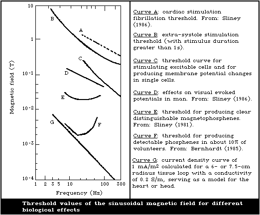 (c) 100 - 1000 mA/m2
It has been shown by a number of research groups that current
densities in this range, which result from electric currents
applied in vitro and in vivo to mammalian central nervous tissue,
can influence neuron excitability without causing direct
stimulation. Much of this work has been carried out using rat
hippocampal slices (Bawin et al., 1975, 1978, 1984, 1986) and
guinea-pig hippocampal slices (Jeffries, 1981). The thresholds for
stimulation of sensory receptors and of nerve and muscle cells may
also lie in this range. It is possible that such stimulation could
be hazardous. An unexpected stimulation of muscle tissue may lead
to a dangerous reaction. Changes in excitability or the direct
stimulation of central nervous tissue may lead to adverse changes
in mental function.
(d) Above 1000 mA/m2
An increased probability of ventricular fibrillation occurs at
current densities above 1000 mA/m2. The probability of this effect
increases with both duration of exposure and current density
magnitude. Continuous (tetanic) muscle contraction may also occur.
In studies where 50/60-Hz electric currents have been applied to
human volunteers via electrodes, tetany of the muscles concerned
with breathing has been produced which, obviously, would be fatal
if prolonged.
A summary of the ranges of induced currents that produce these
possible effects is given in Table 15.
Table 15. Induced current density ranges between 3 and 300 Hz
for producing biological effects
-----------------------------------------------------------
Current density Effects
(mA/m2)
-----------------------------------------------------------
< 1 Absence of established effects
1 - 10 Minor biological effects reported
10 - 100 Well established effects, visual
(magnetophosphenes) and possible nervous
system effects; facilitation of bone
fracture reunion reported
100 - 1000 Changes in central nervous system
excitability established; stimulation
thresholds; possible health hazards
> 1000 Extrasystoles, ventricular fibrillation
possible; definite health hazards
-----------------------------------------------------------
In terms of a health risk assessment, it is difficult to
correlate the internal tissue current densities with the external
magnetic field strengths. Calculation of current densities using
Faraday's law is complicated by the fact that the exact current
paths depend in a complex way on the distribution and the
conducting properties of the body tissues. Current densities
induced in human beings and animals are extremely non-uniform.
Current enhancements have been predicted in the human neck,
axillae, and lower pelvic region for exposure to a horizontal ELF
magnetic field (Kaune & Curley, 1986). There are differences in
the conductivity of the white and grey cerebral matter.
Furthermore, the effective diameter of the current pathways (loops)
is not known. However, using "worst case" assumptions, an
estimate of the order of magnitude for "safe" and dangerous
magnetic field strengths and their frequency dependence can be made
(Bernhardt, 1979, 1985).
The threshold field strengths and induced current densities
required to produce visual effects by exposure to time-varying
magnetic fields have been studied as a function of frequency
(sections 4.2 and 6.1). In addition, the effects of electrical
stimulation on cell membrane potentials, sensory receptors, and
cardiac, nerve and muscle tissues have been characterized as a
function of frequency (section 6.2). The frequency dependence of
the thresholds for the direct electrical stimulation of cells and
tissues, as well as the thresholds for magnetic field generation of
phosphenes and for altering the VEP, have recently been summarized
by Bernhardt (1985). By calculating the magnetic flux density that
would produce current densities in tissues comparable with those
produced by direct electrical stimulation, Bernhardt (1985, 1986)
has constructed a family of curves representing the approximate
threshold field levels necessary to produce electrical stimulation
of cells and tissues by time-varying magnetic fields with a
sinusoidal waveform. These threshold field levels are plotted in
Fig. 8 as a function of frequency in the ELF range. Seven curves
are shown in this figure, including some experimental data as
explained in the caption.
With the possible exception of production of magneto-
phosphenes, over the entire ELF range, the threshold field levels
that produce stimulating effects in various target organs and
tissues are greater than those that induce a current density of 1
mA/m2 in the brain or heart. This observation is consistent with
the results of cell and tissue studies summarized in section 6.3,
which indicate that the threshold current density for which
perturbations are consistently observed is approximately 10 mA/m2.
The values given in Fig. 8 for the current densities are
applicable only to the peripheral regions of the heart or the head.
For zones closer to the centre of the heart or the head (having a
shorter current path), higher strengths of the magnetic field are
necessary to induce the same current densities. From Fig. 8, a
magnetic field strength that is considered not to produce any
biological effect is about 0.4 mT for 50 or 60 Hz. Although some
experimental data fit satisfactorily into Fig. 8, it must be
understood that the figure only gives an idea of the magnitude of
the current density in the body. Mean values were taken as the
basis to determine the distribution of the electric field in the
heart and the head, where the exact current paths are not known.
Local increases in the internal field strength cannot be precluded.
The extent of high local field strengths needs further elucidation
by continued studies.
Safety factors may be defined more precisely only after further
studies. This has to be considered in the case where curve G in
Fig. 8 is used to evaluate human exposure to time-varying magnetic
fields or to provide a basis for discussion on the definition and
determination of personnel exposure limits.
8.3. Conclusions
1. Only a few mechanisms of the interaction of biological tissue
with magnetic fields have been established. Some of the biological
effects data suggest that other mechanisms may play a role, but
these have yet to be confirmed experimentally. Thus, only a
preliminary assessment of the human health risks from exposure to
magnetic fields can be made.
2. A number of lower organisms have shown a remarkable
sensitivity to the earth's magnetic field, because of highly
developed receptors. Similar receptors have not been found in
human beings.
3. For human exposure to static magnetic fields, it is not
possible to make any definitive statement about the safety or
hazard associated with short- or long-term exposure to fields above
2 T. Available knowledge suggests the absence of any measurable
effect of static fields on many major developmental, behavioural,
or physiological parameters in higher organisms. Recent medium-
term (days) studies on exposure of animals to static fields of up
to 2 T have not demonstrated any detrimental effects.
4. From the scientific data base on higher organisms exposed to
magnetic fields, only 4 types of effect can be regarded as
established. The first three may be explained by plausible
mechanisms of interaction and produce a basis for extrapolation to
man. These effects are:
(a) induction of electrical potentials and magnetohydro-
dynamic effects within the circulatory system;
(b) the formation of magnetophosphenes with a time rate
of change of magnetic field exceeding 0.3 T/s at
17 Hz; the effect depends strongly on frequency
(compare Fig. 8);
(c) direct stimulation of nerve and muscle cells by very
short (less than 1 ms) pulses of rapidly changing
magnetic fields (several thousand T/s). Current
densities are estimated to exceed 1000 mA/m2. These
effects are strongly frequency dependent and may
exhibit lower thresholds (100 - 1000 mA/m2) under
more favourable stimulus conditions (10 - 100 Hz).
(d) other cellular and tissue alterations when the
induced current densities exceed approximately 10
mA/m2.
5. For human exposure to time-varying magnetic fields, it seems
reasonable to assume that a health risk assessment can be made on
the basis of significant perturbations of biological functions
caused by electric currents induced by the fields. Available data
suggest that, when current densities less than 10 mA/m2 are induced
in tissues and extracellular fluids, the induction of adverse
health effects is unlikely. However, the possibility of some
perturbing effects occurring following long-term exposure cannot be
excluded.
The time-varying fields that induce currents in the body depend
critically on the waveform and pulse shape. In this regard, the
peak instantaneous current densities appear to be important.
Furthermore, the frequency dependence of effects produced by time-
varying fields has to be taken into consideration.
9. STANDARDS AND THEIR RATIONALES
With advances in technology resulting in increasing numbers of
devices using magnetic fields, the potential for human exposure to
these fields has increased to the point that valid questions are
raised concerning safety.
Except for the USSR (USSR, 1970, 1978, 1985) and the Federal
Republic of Germany (1986), no countries have developed, or are
developing, mandatory standards limiting magnetic field exposure
because, until recently, there was only a small probability of
human exposure to magnetic fields strong enough to cause adverse
health effects. However, with the advent of high-energy
accelerators and fusion reactors using strong magnets, magnetic
levitation systems for transport and, most recently, the
application of magnetic resonance techniques in diagnostic
medicine, serious consideration has been given to developing
exposure limits in various countries.
A safety standard is a general term, incorporating both
regulations and guidelines, and is defined to be a set of
specifications or rules to promote the safety of an individual or
group of people. A regulation is promulgated under a legal statute
and is referred to as a mandatory standard. A guideline generally
has no legal force and is issued for guidance only - a voluntary
standard. Safety standards can specify maximum exposure limits and
other safety rules for personnel exposures, or provide details on
the performance, construction, design, or functioning of a device.
The purpose of this section is to briefly summarize the
existing standards on magnetic fields and to discuss their
scientific basis.
9.1. Static Magnetic Fields
Only a few guidelines limiting occupational exposure to static
magnetic fields have been developed. The limits of human exposure
to static magnetic fields in the USSR, US Department of Energy, and
certain accelerator laboratories in the USA, and the CERN
Accelerator Laboratory in Geneva are summarized in Table 16. Only
one standard (USSR, 1978) has been promulgated to regulate static
magnetic fields. A new DIN-VDE draft electromagnetic field
standard is being discussed in the Federal Republic of Germany
(1986) and this includes 0 Hz magnetic fields.
The earliest static magnetic field guidelines were developed
as an unofficial recommendation in the USSR (Vyalov, 1967).
Clinical investigations (Vyalov et al., 1964; Vyalov & Lisichkina,
1966; Vyalov, 1971, 1974) formed the basis for the Soviet Standard
(USSR, 1978). The standard requires that the static magnetic field
strength at the work-place does not exceed 8 kA/m (0.01 T).
Table 16. Limits of occupational exposure to static magnetic fields
------------------------------------------------------------------------------------------------
Author Field Exposure time Body region Comments
------------------------------------------------------------------------------------------------
USSR (1978) 0.01 T 8 h whole body regulation issued by Ministry of
Health
Stanford 0.02 T extended (h) whole body unofficial, occupational
Linear 0.2 T short (min) whole body
Accelerator 0.2 T extended (h) arms, hands
Center (1970) 2 T short (min) arms, hands
US Department of 0.01 T 8 h whole body recommended to DOE contractors
Energy (DOE) 0.1 T 1 h or less whole body
(Alpen, 1979) 0.5 T 10 min or less whole body
0.1 T 8 h arms, hands
1 T 1 h or less arms, hands
2 T 10 min or less arms, hands
CERN Accelerator 0.2 T minutes whole body Recommended practice
Lab, Geneva 2 T short hands, arms
(NRPB, 1981) and feet
Lawrence 0.06 T day trunk maximum average/day in peak fields
Livermore > 0.5 T
National
Laboratory 0.06 T day trunk maximum average/week in peak fields
(LLNL,1985) < 0.5 T
0.6 T day extremities maximum average/week (in peak fields
< 0.5 T) or per day (in peak fields
> 0.5 T)
2 T short (min) whole body peak exposure limit
------------------------------------------------------------------------------------------------
Three sets of guidelines recommending limits of occupational
exposure to static magnetic fields exist in the USA. Two of these
are applicable in high-energy physics laboratories, and the other
is a US Department of Energy (DOE) guideline.
At the Stanford Linear Accelerator Center in California,
unofficial guidelines were established in 1970. They suggest that
the whole body or head of workers should not be exposed to static
magnetic fields exceeding 0.02 T for extended periods (h) or fields
exceeding 0.2 T to the arms and hands. For short periods (min), the
whole body or head, and arms and hands should not be exposed to
fields exceeding 0.2 and 2 T, respectively. The 2-T limit also
allows film changes at Stanford's bubble chamber.
The Lawrence Livermore National Laboratory (LLNL, 1985) has
drafted a set of policy guidelines for working in magnetic fields
associated with the high-energy accelerators. The guidelines
(Table 16) state that:
Maximum exposure: Workers must never be exposed to fields
exceeding 2 T, regardless of the duration of the exposure
or the exposed part of the body;
Fields less than 500 mT: If the peak field to which
workers are exposed is less than 500 mT, personnel may be
exposed to a week-long maximum average field strength of
no more than 60 mT (measured at the torso) or 600 mT
(measured at the extremities);
Fields greater than 500 mT: If the peak exposure is
greater than 500 mT, workers should be exposed to a daily
maximum average field strength of no more than 60 mT
(measured at the torso) or 600 mT (measured at the
extremities).
In addition, the following restrictions are made: Always use
caution signs indicating the presence of a magnetic field, whenever
the field strength is 1 mT or greater. Use additional
administrative controls or barricades (ropes or fences), whenever
practical. Do not allow workers with cardiac pacemakers or other
medical electronic implants into areas where the magnetic-field
intensity exceeds 1 mT. Magnetic fields greater than this level
can trigger a change in the operating mode of some pacemakers.
Persons with small metallic implants (such as aneurysm clips) must
also be stopped from entering an area where the field intensity is
greater than 1 mT. Stronger magnetic fields may rotate or even
remove aneurysm clips from the arteries to which they are attached.
Workers with large metallic implants, such as hip prostheses,
should be advised to avoid working anywhere inside the perimeter of
1-mT field intensity.
A rationale supporting the guidelines accompanies the document
(LLNL, 1985). The 60-mT limit is set to 1 mV of the
magnetohydnamic voltage (voltage generated by blood, an ionized
fluid, moving in a fixed magnetic field) in an obese person engaged
in moderately heavy work (cardiac output 10 litres/min). 2 T
limits the rise in blood pressure to 1%.
The US Department of Energy (DOE) formed an ad hoc committee to
review technologies that use magnetic fields, to make an assessment
of the scientific literature on biological effects, and to
establish guidelines for static magnetic fields, field gradients,
and time-varying magnetic fields. In July 1979, the Alpen
Committee (Alpen, 1979) made its recommendations to DOE as shown in
Table 16. The guideline in some cases is a factor of 2 lower than
that for continuous exposure at the Stanford Linear Accelerator
Center. This guideline was recommended by the Department of Energy
to its contractor organizations as an interim measure, until
official standards are promulgated. Although the Alpen Committee
made a review of the literature it has not published a rationale
supporting the values recommended in their guideline. According to
Tenforde, the 0.01 T limit was recommended for continuous exposure,
because this represented the accepted threshold for
magnetophosphene production by ELF magnetic fields, and the
threshold for inducing measurable electrical potentials in the
central circulatory system during exposure to static magnetic
fields.
A similarly recommended practice for limiting static magnetic
field exposures of workers exists at the CERN accelerator
laboratory in Geneva (NRPB, 1981). CERN recommends that exposure
of the hands, arms, and feet should not exceed 2 T for periods of
the order of minutes. This is reduced by a factor of 10, if the
head or whole body is exposed.
With the advent of magnetic resonance imaging (MRI), the need
for occupational exposure limits has become more apparent, and
other organizations that traditionally recommend occupational
exposure limits have begun to address this need, despite a
reluctance in the past to recommend limits for magnetic fields
(Sliney, 1986).
9.2. Time-Varying Magnetic Fields
Except for guidelines limiting patient and operator exposure
during clinical magnetic resonance imaging, the only standard
limiting exposure of time-varying magnetic fields in the ELF range
is the Soviet Standard (USSR, 1985), as shown in Table 17. The 50-
Hz magnetic field standard (USSR, 1985) issued by the Ministry of
Public Health of the USSR in January 1985 makes a distinction
between continuous and pulsed fields and limits the duration of
exposure, depending on the pulse characteristics. The limits for
exposure to continuous wave fields equate to 7.5 mT for 1 h and 1.8
mT for 8 h. This standard seems to have been developed for arc
welding, since pulsed field exposure occurs most frequently in
welding. The scientific basis for this standard does not appear to
have been published.
The Federal Republic of Germany (1986) is discussing extention
of its current electromagnetic field standard (Federal Republic of
Germany, 1984) down to 0 Hz.
9.3. Magnetic Resonance Imaging Guidelines
Comparing the magnetic field limits in Table 16 with the
strength of the magnets used in MRI, it is not surprising that
regulatory and health agencies have begun to look more seriously at
this imaging modality (Repacholi, 1986). Hundreds of MRI machines
have been installed throughout the world and concern about their
safety has been expressed (Bore, 1985). Some of these machines use
superconductive magnets with fields for diagnostic application up
to about 2.0 T, and there are prototypes with magnets giving fields
of 4 - 5 T. These prototypes are being studied to determine the
feasibility of in vivo spectroscopy.
During the imaging procedure, lasting up to tens of minutes,
the patient lies on a table and all parts of the body are exposed
to strong static magnetic fields, changing (or time-varying)
magnetic fields and radiofrequency radiation. Rapidly switched
gradient fields are superimposed on the static field to allow
spatial information to be obtained. These time-varying fields
induce electric currents in the body.
Table 18 shows the guidelines on static and time-varying
magnetic field exposure for the clinical examination of patients
during MRI, recommended by the Center for Devices and Radiological
Health (CDRH, 1982) of the US Department of Health and Human
Services, the National Radiological Protection Board (NRPB, 1984)
in the United Kingdom, the Federal Health Office (FHO, 1984) of the
Federal Republic of Germany, and Health and Welfare Canada (Health
and Welfare Canada, 1986).
In January 1984, the Health Council of the Netherlands (HCN,
1984) issued interim advice on the use of magnetic resonance
imaging. This general document contains a section on possible
health risks including statements such as: there are no risks to
health from static magnetic field exposures up to 0.5 T, and even
exposures to fields up to 2 T appear safe. More research is needed
to determine the safety of fields stronger than 2 T. The document
also recommends that limits for time-varying magnetic fields and
radiofrequency fields accepted in the USA (CDRH, 1982) or the
United Kingdom (NRPB, 1981) should be followed.
Table 17. Maximum permissible levels of magnetic fields with a
frequency of 50 Hza
---------------------------------------------------------------------------
Duration Magnetic field strength A/m
of Continuous and Pulsed magnetic Pulsed magnetic
exposure pulsed magnetic field field
(h) fields with pulse 60 s > tw > 1 s 0.02 s < tw < 1 s
width tw > 0.02 s tp > 2 s tp > 2 s
and pause tp < 2 s
---------------------------------------------------------------------------
1 6000 8000 10 000
1.5 5500 7500 9500
2 4900 6900 8900
2.5 4500 6500 8500
3 4000 6000 8000
3.5 3600 5600 7600
4 3200 5200 7200
4.5 2900 4900 6900
5 2500 4500 6500
5.5 2300 4300 6300
6 2000 4000 6000
6.5 1800 3800 5800
7 1600 3600 5600
7.5 1500 3500 5500
8 1400 3400 5400
---------------------------------------------------------------------------
a From: USSR (1985).
Note: The above regimes of pulsed exposures are used in welding.
tw is the pulse width duration.
tp is the pulse pause duration.
Magnetic flux density in mT = Magnetic field strength
in A/m x 1.256
103
Table 18. Guidelines on magnetic field exposure in clinical MR
---------------------------------------------------------------------------
Country Static fields Time-varying fields
---------------------------------------------------------------------------
USA Patient - 2 T whole and Patient - 3 T/s whole and partial
CDRH partial body exposure body exposure
(1982)
Exposure exceeding these limits should be evaluated on an
individual basis
United Operator - 0.02 T (long Patient and volunteers - 20 T/s
Kingdom periods, whole body); (rms) periods of magnetic
NRPB 0.2 T (long periods, field change > 10 ms
(1984) arms, hands);
0.2 T (15 min, whole or
body)
2 T (15 min, arms, (dB/dt)2t < 4 (rms) for dura-
hands) tion of magnetic field change
< 10 ms where dB/dt in T/s and
t in s
Patient and volunteers -
2.5 T (whole and partial
body exposure)
Germany, Patient - 2 T (whole and Patient - whole and partial body
Federal partial body exposure) exposure: maximum induced current
Republic of density
FHO (1984) 30 mA/m2 or 0.3 V/m electric
field strength for duration of
magnetic field change of 10 ms
or longer
or
(300/t) mA/m2 or (3/t) V/m for
duration of magnetic field change
(t) shorter than 10 ms (t in ms)
Canada Operator - 0.01 T (whole Patient - 3 T/s (rms)
Health and body during working day)
Welfare
Canada - > 0.01 T
(1986) (keep to minimum)
Patient - 2 T (whole and
partial body exposure)
---------------------------------------------------------------------------
9.3.1 United Kingdom
The NRPB (1984) recommends that the following conditions should
be fulfilled during the operation of magnetic resonance imaging
equipment in the United Kingdom.
(a) Static fields
For people (patients and volunteers) exposed to the imaging
process, the static magnetic field should not exceed 2.5 T for the
whole or a substantial portion of the body. The NRPB Advisory
Group formulating the guidelines suggested that static fields have
been shown to affect certain chemical reactions in vitro and that
reproducible changes in primate behaviour have been found in fields
of several tesla. Although flow potentials are generated across
blood vessels by the flow of blood perpendicular to the field,
their biological significance at fields of a few tesla remains
unclear. However, at 2.5 T, the peak flow potential is calculated
to be approaching the depolarization threshold for myocardial
muscle. Although only a fraction of this potential occurs across
each cell, it was considered prudent to limit acute exposure to 2.5
T, until further information becomes available.
Occupational static field exposure limits are recommended for
staff operating MRI equipment. Exposure for prolonged periods to
more than 0.02 T for the whole body or 0.2 T for the arms or hands
should be avoided. NRPB (1984) recommends that these limits may be
increased to 0.2 T for the whole body and 2 T for the arms and
hands for periods totalling less than 15 min at a time, provided
intervals of about 1 h occur between such exposures.
These operator limits are essentially the same as those
recommended by the Stanford Linear Accelerator Center (Table 16),
where no adverse symptoms have been reported from staff working at
the facility, since the introduction of their guidelines in 1970.
(b) Time-varying fields
For the time-varying fields, excluding radiofrequency fields,
the NRPB (1984) recommends limits based on the duration of magnetic
flux density changes (i.e., the time during which electric currents
are being induced). When the duration of exposure exceeds 10 ms,
exposures should not exceed root mean square (rms) rates of change
of magnetic flux density (dB/dt) of 20 T/s for all persons
(patients exposed to the imaging process, volunteers). For
durations of change of less than 10 ms, the relationship (dB/dt)2t
less than 4 should be observed where dB/dt is in T/s, and t is the
duration of the change of the magnetic field in seconds. For
continuously varying magnetic fields, such as sinusoidal fields,
the duration of the change can be considered as half the period of
the waveform.
The rationale for the NRPB guidelines is given in a publication
by Saunders & Smith (1984). The NRPB Advisory Group recognized
that rapidly changing magnetic fields can induce electric currents
in tissues that could be sufficiently large to interfere with the
normal functioning of nerve cells and muscle fibres. These conduct
electrical impulses in the form of localized membrane
depolarization produced by the flow of ions and, above a certain
threshold, give rise to sensation or muscle contractions. From
experimental data it was inferred that the threshold would be
lowest when the current pulse width (or duration of magnetic flux
density change) exceeded about 10 ms.
It was felt that, although the sensation of magnetic phosphenes
occurred at a threshold in man of about 1.3 T/s (at 20 Hz), this
sensation of light flashes in the eye has not been shown to be
hazardous. However, excitation of nerves and muscles could be
hazardous, but requires exposure to high rates of change of
magnetic flux density. The threshold for excitation depends on the
pulse length and pulse repetition frequency of the induced current.
Since insufficient information is available to define safe limits,
they must be derived from effects of electric currents applied by
electrodes. The threshold current density to induce ventricular
fibrillation is 3 A/m2. Thus, to achieve a factor of 10 safety
margin, it was decided that MRI operating conditions should be such
as to induce current densities that did not exceed 0.3 A/m2 for a
duration of magnetic flux density change greater than 10 ms.
For durations of the current pulse of half period (t) of less
than 10 ms, the evidence suggests that, when t decreases, the
threshold rms current density for inducing ventricular fibrillation
increases. Experimental data suggest that the square of the rms
current density multiplied by the duration (t) remains constant.
The magnetic field vector in most MRI equipment is parallel to the
longitudinal axis of the body (z-axis). The current density
induced by time variation of the z-gradient is proportional to the
conductivity, the inductive loop radius, and the rate of change of
the magnetic field. Assuming the average value for tissue
conductivity to be 0.2 S/m, the radius of the body to be 0.15 m,
the limit applied to the rms current density of 0.3 A/m2 for pulses
or half periods of induced current exceeding 10 ms restricts the
rms rate of change of the z gradient magnetic flux density to 20
T/s, when the duration of magnetic field change exceeds 10 ms. For
durations shorter than 10 ms, (Saunders & Smith, 1984), the
relationship for determining the limit for the time-varying field
can be derived:
(dB/dt)2t < 4,
where dB/dt is in T/s, and t is in seconds
It was assumed that the current densities induced in the body
by variation of the anterior-posterior (y) and lateral (x)
gradients would not be significantly greater than for the z
gradients.
(c) Other guidelines
(i) RF exposure of the patient and staff must be
restricted so that the rise in temperature does not
exceed 1 °C, as shown by skin and rectal temperature,
or more than 1 °C in any mass of tissue not exceeding
1 g in the body.
(ii) Patients should be exposed only with the approval
of a registered medical practitioner or research
ethics committee.
(iii) Patients must be fully informed of the procedure
and consent freely to it.
(iv) Only medically assessed suitable volunteers should
be used in trials.
(v) Frequently exposed volunteers should have regular
ECG checks.
(vi) It is prudent to exclude women in the first three
months of pregnancy.
(vii) Special care is needed for patients with cardiac
pacemakers or large metallic implants.
(viii)Warning notices should be posted indicating that
magnetic and RF fields may affect pacemakers and
electronic equipment.
9.3.2 USA
The recommendations issued by the Center for Devices and
Radiological Health (CDRH, 1982) in the USA are intended to assist
the medical profession and manufacturers in making health risk
benefit assessments. Based on information available in the
literature, it was suggested that, in the case of diagnostic
magnetic resonance applications involving exposure to static
magnetic fields not exceeding 2 T or time-varying fields not
exceeding 3 T/s, the benefits outweigh the risks, within the
current medical indications and contra-indications. Pregnant women
should not be exposed as the safety of such exposure has not been
established. It should be noted that the CDRH guidelines are not
limits for patient exposure in MRI imaging investigations. The
recommendations are essentially criteria that provide a demarcation
between devices exceeding the magnetic field levels stated in the
guidelines and therefore requiring further evaluation to determine
if any health risk exists for the patient, and devices operating
below the levels given in the guidelines.
The recommendations for the magnetic field levels were
determined after consideration of existing unofficial standards and
recommendations and their rationales, and a review of the
scientific literature. The scientific rationale for the guidelines
is essentially that proposed by Budinger (1981). Budinger
concluded, after a review of the bioeffects literature and a
theoretical analysis of the known interaction mechanisms of static
magnetic fields with biological systems, that harmful effects on
human beings or reproducible cellular, biochemical, and genetic
effects have not yet been observed and are not expected at fields
of less than 2 T. For changing magnetic fields, Budinger concluded
that the thresholds for effects of induced currents is above that
produced by 1 - 100 Hz sinusoidal fields of strength 5 mT. However,
he did note that potential biological effects due to differences in
waveform, repetition rate, peak magnetic field, and duration of
exposure required further study.
The CDRH also recommends that the radiofrequency field exposure
of the patient should be limited, so that the specific absorption
rate (SAR) does not exceed 0.4 W/kg, averaged over the whole body,
or 2 W/kg, averaged over any gram of tissue.
9.3.3 Federal Republic of Germany
The Federal Health Office (FHO, 1984) has made recommendations
to physicians who work with clinical MRI devices. It is stated that
no adverse health effects on patients, operators, or any other
persons in the vicinity of MRI equipment have been detected so
far. However, possible effects on the body can be estimated from
induced currents and potentials in the body. The guidelines for
static and time-varying magnetic fields are based on these
estimations and study of the literature. It is stated that, if
there is compliance with these recommendations, any detrimental
effects will be detected at the earliest possible time. A
translation of the original guidelines from German to English is
provided in Bernhardt & Kossel (1985).
(a) Static fields
The FHO recommends that patients imaged in an MRI facility
should not be exposed to static magnetic fields exceeding 2 T. If
patients are exposed to fields higher than 2 T, they should be
monitored for cardiac and circulatory function.
The rationale for determining this value is as follows:
orientation effects are observed in such systems as DNA, retinal
rods, and sickle cells at static field strengths above 1 - 2 T.
Electric potentials induced in flowing blood exposed to static
fields above 0.3 T have been noted in ECG measurements in animals,
but no adverse health effects have been observed in animals exposed
to fields up to 10 T. However, the potential differences induced
by cardiac contractions in a magnetic field exceeding 2 T may impair
the excitation stimulation or conduction of excitation.
(b) Time-varying fields
Time-varying magnetic fields induce electrical potentials, the
size of which depends on the magnetic field strength, pulse
duration and frequency. Using essentially the reasoning outlined
by Bernhardt (1985) for estimating the values of induced electric
potentials and currents that are likely to cause biological
effects, the FHO (1984) recommends that patients should not be
exposed to time-varying magnetic fields having a duration of
magnetic field change equal to or greater than 10 ms, which induce
electric fields greater than 0.3 V/m or current densities exceeding
30 mA/m2. If the duration of the magnetic field change of the
time-varying fields is less than 10 ms, then the maximum induced
electric field is 3/t V/m and maximum induced current density is
300/t mA/m2 (0.3/t A/m2), where t is the duration of magnetic field
change in milliseconds. The MRI machine manufacturer must inform
the purchaser of the operating conditions that will result in the
induced field strength and current density remaining below the
recommended values. If these values are capable of being exceeded
by the machine, the manufacturer must prove that it is safe.
A brief rationale for these recommended values is given in FHO
(1984). Compared with natural currents, induced current densities
of 1 mA/m2 have no detectable effect on the body. Current densities
of 10 mA/m2 induce effects that depend on the frequency of the
time-varying magnetic field, but do not pose hazards. At
frequencies between 10 and 50 Hz, magnetic fields above 5 mT
produce magnetophosphenes. Ventricular fibrillation may be caused
if the magnetic field induces current densities exceeding 1000
mA/m2 or electric fields exceeding 100 mV/cm.
The final values of induced electric field and current density
represent estimates, based on studies and theoretical calculations
(described by Bernhardt, 1985), that are thought to provide a wide
margin of safety.
(c) Other recommendations
1. Exposure to radiofrequency fields should be such that
the SAR does not exceed 1 W/kg (whole body) or 5 W/kg
(partial body - per kg of tissue, except the eyes).
2. Prior to patient examination, care must be taken with
regard to implants made of ferromagnetic materials,
implanted cardiac pacemakers, dislocation of catheters,
vascular clips, and the like.
3. Patients must undergo additional medical examinations
(described in FHO, 1984), if the recommended exposure
limits are exceeded.
9.3.4 Canada
The Bureau of Radiation and Medical Devices of Health and
Welfare Canada (Health and Welfare Canada, 1986) has published a
safety code containing guidelines on exposure to electromagnetic
fields from magnetic resonance clinical systems. The document
contains information on levels of exposure for typical devices,
exposure guidelines from various countries, a summary of health
effects from magnetic and radiofrequency fields, and guidance on
exposure of patients and operators. Details of the guidelines are
given in Table 18.
Health and Welfare Canada (1985) have also published
recommendations to ensure the protection of patients and
operational personnel from potential hazards in MRI. This report
contains recommendations on magnetic fields as shown below:
(a) static magnetic fields must be below 0.5 mT in
unrestricted areas;
(b) entrance to areas in excess of 1.5 mT must be
strictly controlled, to prevent introduction of
magnetic material by patients, operational personnel,
and visitors;
(c) equipment for cardiopulmonary resuscitation must be
available and usable within the imaging room and, if
possible, in areas where the field exceeds 10 mT;
(d) static magnetic fields should not exceed 2.5 T (this
differs from the 2 T recommended in Health and
Welfare Canada (in press)); and
(e) time-varying magnetic fields should not exceed 3 T/s.
10. PROTECTIVE MEASURES AND ANCILLARY HAZARDS
Protective measures for the industrial and scientific use of
magnetic fields can be categorized as engineering design measures,
the use of separation distance, and administrative controls.
Another general category of hazard control measures, namely
personal protective equipment (e.g., special garments and face
masks) do not exist for magnetic fields. However, protective
measures against ancillary hazards from magnetic interference with
emergency or medical electronic equipment and for surgical and
dental implants are a special area of concern regarding health
aspects of magnetic fields. The mechanical forces imparted to
ferromagnetic implants and loose objects in high-field facilities
require that precautions be taken.
The techniques to minimize needless exposure to high intensity
magnetic fields around large research facilities generally fall
into three types:
(a) Distance and time
Limit human access and/or occupancy duration in locations where
field strengths are high. Since the external magnetic flux density
decreases with distance from the source, separation distance is a
fundamental protective measure. For example, at large distances
from a static magnetic field dipole source, the field decreases
approximately as the reciprocal cube of the separation distance.
(b) Magnetic shielding
The use of ferromagnetic core materials restricts the spatial
extent of external flux lines of a magnetic device. External
enclosures of ferromagnetic materials can also "capture" flux lines
and reduce external flux densities. However, shielding is normally
an expensive control measure and of limited use for scientific
instruments. Furthermore, it has not generally been shown to be
cost-effective for large installations when compared to the use of
separation distance (Hassenzahl et al., 1978).
(c) Electromagnetic interference (EMI) and cardiac pacemakers
Certain types of modern cardiac pacemakers exhibit malfunction
in response to EMI produced either by endogenous myopotentials or
by external sources such as high-voltage systems. The modern
implantable pacemakers are microprocessor-controlled and function
in a "demand" mode in which stimulatory pulses are delivered to
the heart, only if it fails to exhibit intrinsic electrical
activity. The endogenous cardiac activity is detected by a signal-
sensing circuit, in order to avoid competitive pacing between the
pacemaker's stimuli and the heart's intrinsic activity. The modern
pacemakers also contain a noise detection circuit that can
discriminate electric fields with different frequencies and
waveforms from those associated with the heart's bioelectrical
activity. When EMI is sensed, the demand pacemaker reverts to a
fixed-rate pacing mode, which may be asynchronous with the normal
cardiac activity. This pacing mode is frequently referred to as
the "reversion" or "noise" mode of operation, and can be
undesirable if the pacemaker signals are competitive with the
intrinsic cardiac electrical activity.
Two different configurations of electrode leads are used in
pacemakers, and these have very different sensitivities to EMI. In
one type, termed the "bipolar" design, both leads are implanted
within the heart at a typical separation distance of 3 cm. In the
second type, termed the "unipolar" design, the cathode lead is
implanted in the heart and the pacemaker case serves as the anode.
Because of the considerable physical separation of the anode and
cathode leads in the unipolar design, this type of pacemaker
provides a large antenna for the reception of EMI. Of the two
designs for pacemaker electrode configurations, only the unipolar
type has been found to be sensitive to EMI. Among the 350 000 -
500 000 individuals in the USA who have implanted pacemakers,
approximately 50% have models with the unipolar electrode design.
During the past decade, several laboratory tests and studies on
pacemaker patients have been conducted to assess the response of
different pacemaker models to power-frequency electric and magnetic
fields (Jenkins & Woody, 1978; Butrous et al., 1983; Griffin, 1985;
Moss & Carstensen, 1985). Two types of pacemaker malfunction have
been observed in response to EMI: (a) an aberrant pacing rate, with
irregular or slow pacing; and (b) reversion to fixed-rate
(asynchronous) pacing. The probability that a malfunction will
occur in the presence of an external electromagnetic field is
strongly dependent on the pacemaker model, since some manufacturers
have incorporated a feature into their pacemaker models that
automatically decreases the sensitivity of the amplifier circuit
when EMI is sensed. These specific brands of pacemaker thereby
avoid reversion to an asynchronous mode in response to EMI.
Griffin (1985) estimated the total population of pacemaker
patients in the USA who might be at serious risk from the effects
of EMI. He assumed that: (a) 350 000 - 500 000 individuals wear
pacemakers; (b) 50% of the pacemakers are of the unipolar design;
(c) 10 - 20% of the unipolar pacemakers are highly sensitive to
EMI; and (d) 20 - 25% of the patients with sensitive pacemakers are
totally dependent on the pacemaker to sustain their cardiac
rhythm. With these assumptions, it can be calculated that
approximately 3500 - 12 000 pacemaker wearers might be at serious
risk from EMI. However, it must be borne in mind that only a small
fraction of the individuals at risk are likely to encounter a
source of EMI during the time periods when their cardiac function
is totally dependent on an implanted pacemaker. The above estimate
of the population at risk must therefore be regarded as an upper
limit that perhaps greatly overestimates the actual probability of
the occurrence of a potentially fatal pacemaker malfunction in
response to EMI.
Both power-frequency electric and magnetic fields have been
found to introduce EMI that can alter the functioning of many
commercially available pacemakers. In studies on 11 patients with
7 different implanted pacemaker models from 4 manufacturers, Moss &
Carstensen (1985) observed alterations in pacemaker function during
exposure to 60-Hz electric fields ranging from 2 - 9 kV/m. Only
models produced by 2 out of the 4 manufacturers were sensitive to
EMI from fields of this strength. A similar set of observations
was made by Butrous et al. (1983).
A total of 26 pacemaker models were examined by Jenkins & Woody
(1978). Twenty of these units were found to revert to an
asynchronous mode of pacing or to exhibit abnormal pacing
characteristics in 60-Hz fields ranging from 0.11 to 0.4 mT, with
the average threshold field level for an effect being 0.21 mT. The
minimum value of dB/dt producing an effect was therefore 41.5 mT/s
(for the 60-Hz, 0.11-mT field). Pacemaker malfunctions produced by
power-frequency magnetic fields require field levels that are
greater than those associated with high-voltage transmission lines
and most other types of electrical systems. However, the fields in
the immediate vicinity of various types of industrial machinery and
appliances (section 3) are sufficiently strong to represent a
potential source of EMI that could alter pacemaker functioning.
Pavlicek et al. (1983) found that a rapidly switched gradient
field used in magnetic resonance imaging with a time variation of 3
T/s could induce potentials up to 20 mV in the loop formed by the
electrode lead and the case of a unipolar pacemaker. This signal
amplitude is sufficiently large to avoid rejection by the
pacemaker's EMI discrimination circuitry, and could therefore be
recognized as a valid cardiac signal.
Pacemaker malfunctions can also be caused by static magnetic
fields, which produce closure of a reed relay switch used to test
the pacemaker's performance while operating in a fixed rate pacing
mode. On the basis of a study of pacemakers produced by 6 major
manufacturers, Pavlicek et al. (1983) found the most sensitive
model to exhibit reed switch closure and reversion to fixed-rate
pacing in a 1.7-mT static field. Field levels of 1.7 - 4.7 mT were
observed to produce closure of the reed switches in all of the
models tested. All of the models were also found to experience
forces and torques when placed in MRI devices operated at fields of
up to 0.5 T. Two of the pacemakers experienced a torque that was
strong enough to produce significant movement of these units within
tissue.
(d) Administrative measures
The use of warning signs, and special access areas to limit
exposure of personnel near large magnet facilities has been of
greatest use to control exposure. Administrative controls, such as
these, are generally preferable to using magnetic shielding, which
can be extremely expensive. In some circumstances, for example MRI
facilities, a combination of shielding, restricted access, and the
use of metal detectors may be appropriate to avoid detrimental
effects from exposure to high strength magnetic fields. Loose
ferromagnetic and paramagnetic objects can be converted into
dangerous missiles when subjected to intense magnetic field
gradients. Avoidance of this hazard can only be achieved by
removing loose metallic objects from the area and personnel. Such
items as scissors, nail files, screwdrivers, and scalpels should be
banned from the immediate vicinity.
Of particular concern in MRI, are the forces exerted by static
magnetic fields on implanted metal objects such as aneurysm clips
and pacemakers. Even the most modern pacemakers will malfunction
when placed in an MRI machine (Erlebacher et al., 1986). New et
al. (1983) also measured the magnetic torques exerted on 21 types
of haemostatic clips and various other materials such as dental
amalgam. Of the 21 clips, 19 of which were aneurysm clips, 16
showed a deflection near the portals of two magnets operating at
0.147 T and 1.44 T, respectively. Of the remaining materials
tested, only a shunt connector demonstrated significant
ferromagnetic properties. The non-magnetic materials were
primarily composed of austenitic stainless steel. Surgical clips
composed of tantalum or titanium are also non-ferromagnetic. Clips
composed of martensitic stainless steels are ferromagnetic and
experience significant forces and torques in static magnetic
fields. These findings indicate a clear requirement for strict
administrative controls in determining whether patients bearing
medical implants could be adversely affected by the fields present
in MRI devices.
REFERENCES
AARHOLT, E., FLINN, E.A., & SMITH, C.W. (1981) Effects of
low-frequency magnetic fields on bacterial growth rate. Phys.
biol. Med., 26: 613-621.
AARHOLT, E., FLINN, E.A., & SMITH, C.W. (1982) Magnetic
fields affects the Lac operon system. Phys. biol. Med., 27:
606-610.
ABASHIN, V.M. & YEVTUSHENKO, G.I. (1984) The mechanisms of
biological effects of low frequency electromagnetic fields in
the biosphere. In: Biological effects of electromagnetic
fields, Moscow, Nauka, Vol. 2, pp. 193-201.
ABRAMOVICH-POLJAKOV, D.K., KLEINER, A.I., KOLODUB, F.A.,
KRAKOVSKAYA, S.P., NEDBAILS, E.P., PENOVA, V.N., SMOLJANOVA,
N.S., TRIKOZA, V.A., & STEINGERZ, L.A. (1979) [Clinical
characteristics of effects of electromagnetic fields from
contact welding.] Vrach. Delo, 4: 106-119 (in Russian).
ACETO, H., Jr, TOBIAS, C.A., & SILVER, I.L. (1970) Some
studies on the biological effects of magnetic fields. IEEE
Trans. Mag., 6: 368-373.
ADEY, W.R. (1980) Frequency and power windowing in tissue
interactions with weak electromagnetic fields. Proc. IEEE, 68:
119-125.
ADEY, W.R. (1981) Tissue interactions with non-ionizing
electromagnetic fields. Physiol. Rev., 61: 435-514.
ADEY, W.R. (1983) Some fundamental aspects of biological
effects of extremely low frequency (ELF). In: Grandolfo, M.,
Michaelson, S.M., & Rindi, A., ed. Biological effects and
dosimetry of non-ionizing radiation, New York, London, Plenum
Press, 561-580.
AKOYUNOGLOU, G. (1964) Effect of a magnetic field on
carboxydismutase. Nature (Lond.), 202: 452-454.
ALEKSANDROV, M.S., BAKLENEVA, A.M., GLADSTEIN, N.D., OZEROV,
V.P., POTAPOV, A.V., & REMIZOV, L.T. (1972) [Fluctuations of
the earth's electromagnetic field,] Moscow, Nauka, p. 195 (in
Russian).
ALPEN, E.L. (1979) Magnetic field exposure guidelines. In:
Tenforde, T.S., ed. Magnetic field effects on biological
systems, New York, London, Plenum Press, pp. 25-32.
AMER, N.M. (1965) The effects of homogeneous magnetic
fields, ambient gas composition, and temperature on
development of Tribolium confusum, Berkeley, University of
California, Lawrence Radiation Laboratory (Report No.
UCRL-16854).
AMERICAN INSTITUTE OF BIOLOGICAL SCIENCES (1985) Biological
and human health effects of extremely low frequency
electromagnetic fields, Arlington, Virginia, American
Institute of Biological Sciences, p. 290.
AMINEV, G.A., AMINEVA, R.I., & SITKIN, M.I. (1967) [The
influence of magnetic fields on the learning process of mice
in a T-shaped maze.] In: [Problems of bionics,] Moscow, Nauka,
pp. 338-340 (in Russian).
ANDRIANOVA, L.A. & SMIRNOVA, N.P. (1977) [Motor activity of
muscles in a magnetic field of varying intensity.] Kosm. biol.
aviakosm. Med., 11: 54-58 (in Russian).
ANIOLCZYK, R. (1981) Measurements and hygienic evaluation of
electromagnetic fields in the environment of diathermy,
welders, and induction heaters. Med. Pracy, 32: 119-128.
ANTONOWICZ, K. (1974) Possible superconductivity at room
temperature. Nature (Lond.), 247: 358-360.
ARCHER, C.W. & RATCLIFFE, N.A. (1983) The effects of pulsed
magnetic fields on chick embryo cartilaginous skeletal
rudiments in vitro. J. exp. Zool., 225: 243-256.
ARNOLD, W., STEEL, R., & MUELLER, H. (1958) On the magnetic
asymmetry of muscle fibres. Proc. Natl Acad. Sci. (USA), 44:
1-11.
ASANOVA, T.P. & RAKOV, A.I. (1966) [The state of persons
working in electrical fields of outdoor 400- and 500-kV
switchyards.] Gig. Tr. Prof. Zabol., 10: 50-52 (in Russian).
BAKER, R.R. (1980) Goal orientation by blindfolded humans
after long distance displacement: possible involvement of a
magnetic sense. Science, 210: 555-557.
BAKER, R.R., MATHER, J.G., & KENNAUGH, J.H. (1983) Magnetic
bones in human sinuses. Nature (Lond.), 310: 78-80.
BARKER, A.T., DIXON, R.A., SHARRAD, W.J.W., & SUTCLIFFE, U.L.
(1984) Pulsed magnetic field therapy for tibial non-union.
Interim results of a double-blind trial. Lancet, 1: 994-996.
BARLOW, H.B., KOHN H.I., & WALSH, E.G. (1947a) The effect of
dark adaption and of light upon the electric threshold of the
human eye. Am. J. Physiol., 148: 376-381.
BARLOW, H.B., KOHN, H.I., & WALSH, E.G. (1947b) Visual
sensations aroused by magnetic fields. Am. J. Physiol., 148:
372-375.
BARNOTHY, J.M. (1964a) Development of young mice, In:
Barnothy, M.F., ed. Biological effects of magnetic fields, New
York, London, Plenum Press, Vol. 1, pp. 93-99.
BARNOTHY, J.M. (1964b) Rejection of transplanted tumors in
mice. In: Barnothy, M.F., ed. Biological effects of magnetic
fields, New York, London, Plenum Press, Vol. 1, pp. 100-108.
BARNOTHY, J.M., BARNOTHY, M.F., & BOSZORMENYI-NAGY, I.
(1956) Influence of a magnetic field upon the leukocytes of
the mouse. Nature (Lond.), 177: 577-578.
BARNOTHY, M.F., ed. (1964) Biological effects of magnetic
fields, New York, London, Plenum Press, Vol. 1, p. 324.
BARNOTHY, M.F., ed. (1969) Biological effects of magnetic
fields, New York, London, Plenum Press, Vol. 2, p. 314.
BARNOTHY, M.F. & SUMEGI, I. (1969a) Effects of the magnetic
field on internal organs and the endocrine system of mice. In:
Barnothy, M.F., ed. Biological effects of magnetic fields, New
York, New York, London, Plenum Press, Vol. 2, pp. 103-126.
BARNOTHY, M.F. & SUMEGI, I. (1969b) Abnormalities in organs
of mice induced by a magnetic field. Nature (Lond.), 221:
270-271.
BARREGARD, L., JARVHOLM, B., & UNGETHUM, E. (1985) Cancer
among workers exposed to strong static magnetic fields.
Lancet, 2(8460): 892.
BASSETT, C.A.L. (1982) Pulsing electromagnetic fields: a new
method to modify cell behaviour of calcified and non-calcified
tissues. Calcif. Tissue Int., 34: 1-8.
BASSETT, C.A.L., PAWLUK, R.J., & PILLA, A.A. (1974)
Augmentation of bone repair by inductively coupled
electromagnetic fields. Science, 184: 575-577.
BASSETT, C.A.L., PILLA, A.A., & PAWLUK, R.J. (1977) A
non-operative salvage of surgically resistant pseudoarthroses
and non-unions by pulsing electromagetic fields. Clin. Orthop.
relat. Res., 124: 128-143.
BASSETT, C.A.L., MITCHELL, S.N., & GASTON, S.R. (1982)
Pulsing electromagnetic field treatment in ununited fractures
and failed arthrodeses. J. Am. Med. Assoc., 247: 623-628.
BATKIN, S. & TABRAH, F.L. (1977) Effects of alternating
magnetic field (12 Gauss) on transplanted neuroblastoma. Res.
Commun. chem. Pathol. Pharmacol., 16: 351-362.
BATTOCLETTI, J.H., SALLES-CUNHA, S., HALBACH, R.E., NELSON,
J., SANCES, A., Jr, & ANTONICH, F.J. (1981) Exposure of
rhesus monkeys to 20 000G steady magnetic field: effect on
blood parameters. Med. Phys., 8: 115-118.
BAUM, J.W., SCHAIRER, I.A., & LINDAHL, K.L. (1979) Tests in
the plant Tradescantia for mutagenic effects of strong fields.
In: Tenforde, T.S., ed. Magnetic field effects on biological
systems, New York, London, Plenum Press, pp. 22-24.
BAWIN, S.M. & ADEY, W.R. (1976) Sensitivity of calcium
binding in cerebral tissue to weak environmental electric
fields oscillating at low frequency. Proc. Natl. Acad. Sci.
(USA), 73: 1999-2004.
BAWIN, S.M., KACZMAREK, L.K., & ADEY, W.R. (1975) Effects of
modulated VHF fields on the central nervous system. Ann. N.Y.
Acad. Sci., 247: 74-81.
BAWIN, S.M., SHEPPARD, A., & ADEY, W.R. (1978) Possible
mechanisms of weak electromagnetic field coupling in brain
tissue. Bioelectrochem. Bioenergy, 5: 67-76.
BAWIN, S.M., SHEPPARD, A.R., MAHONEY, M.D., & ADEY, W.R.
(1984) Influences of sinusoidal electric fields on
excitability in rat hippocampal slice. Brain Res., 323:
227-237.
BAWIN, S.M., SHEPPARD, A.R., MAHONEY, M.D., ABU-ASSAL, M., &
ADEY, W.R. (1986) Comparison between the effects of
extracellular direct and sinusoidal currents on excitability
in hippocampal slices. Brain Res., 362: 350-354.
BECKER, J.F., GEACINTOV, N.E., VAN NOSTRAND, F., & VAN METTER,
R. (1973) Orientation of chlorophyll in vivo. Studies with
magnetic field oriented Chlorella. Biochem. biophys. Res.
Commun., 51: 597.
BECKER, J.F., GEACINTOV, N.E., & SWENBERG, C.E. (1978a)
Photovoltages in suspensions of magnetically oriented
chloroplasts. Biochim. Biophys. Acta, 503: 545-554.
BECKER, J.F., TRENTACOSTI, F., & GEACINTOV, N.E. (1978b) A
linear dichroism study of the orientation of aromatic protein
residues in magnetically oriented bovine rod outer segments.
Photochem. Photobiol., 27: 51-54.
BECKER, VON, G. (1979) The influence of local geomagnetic
and other physical conditions on various insects in an
experimental area. Ztg angew. Zool., 66: 391-416.
BEISCHER, D.E. (1962) Human tolerance to magnetic fields.
Astronautics, 42: 24-25.
BEISCHER, D.E. (1969) Vectorcardiogram and aortic blood flow
of squirrel monkeys (Saimiri sciureus) in a strong super-
conductive electromagnet. In: Barnothy, M., ed. Biological
effects of magnetic fields, New York, London, Plenum Press,
Vol. 2, pp. 241-259.
BEISCHER, D.E. & BREHL, R.J. (1975) Search for effects of
45-Hz magnetic fields on liver triglycerides in mice,
Pensacola, Florida, Naval Aerospace Medical Research
Laboratory (Report No. NAMRL-1197).
BEISCHER, D.E. & KNEPTON, J.C., Jr (1964) Influence of
strong magnetic fields on the electrocardiogram of squirrel
monkeys ( Saimiri sciureus). Aerosp. Med., 35: 939-944.
BEISCHER, D.E. & KNEPTON, J.C., Jr (1966) The
electroencephalogram of the squirrel monkey (Saimiri sciureus)
in a very high magnetic field, Pensacola, Florida, Naval
Aerospace Medical Research Laboratory (NASA Order No. R-39).
BEISCHER, D.E., GRISSETT, J.D., & MITCHELL, R.R. (1973)
Exposure of man to magnetic fields alternating at extremely
low frequency, Pensacola, Florida, Naval Aerospace Medical
Research Laboratory (Report No. NAMRL-1180).
BELLOSSI, A. (1983) No effect of a static uniform magnetic
field on mouse trypanosomiasis. Radiat. environ. Biophys., 22:
311-313
BELLOSSI, A., SUTTER-DUB, M.TH., & SUTTER, B.CH.J. (1984)
Effects of constant magnetic fields in rats and mice: a study
of weight. Aviat. Space environ. Med., 55: 725-730.
BELTRAME, F., CHIABRERA, A., GRATTAROLA, M., GUERINI, P.,
PARODI, G., PONTA, D., VERNAZZA, G., & VIVANI, R. (1980)
Electromagnetic control of cell function. Alta Freq., 49:
101-114.
BENKOVA, N.P. (1975) The magnetic field of the earth and its
variation. In: Physical, mathematical and biological problems
of effects of electromagnetic fields and ionization of air,
Moscow, Nauka, pp. 13-24.
BERNHARDT, J. (1979) The direct influence of electromagnetic
fields on nerve and muscle cells in man within the frequency
range of 1 Hz and 30 MHz. Radiat. environ. Biophys., 16:
309-329.
BERNHARDT, J.H. (1985) Evaluation of human exposures to low
frequency fields In: The impact of proposed radiofrequency
radiation standards on military operations, Neuilly-sur-Seine,
North Atlantic Treaty Organization, pp. 8.1-8.18, (AGARD
Lecture Series No. 138).
BERNHARDT, J.H. (1986) Assessment of experimentally observed
bioeffects in view of their clinical relevance and the
exposure at work places. In: Bernhardt, J., ed. Biological
effects of static and extremely low frequency magnetic fields,
Munich, MMV Medizin Verlag, pp. 157-168.
BERNHARDT, J.H. & KOSSEL, F. (1984) [Health risks from
NMR-tomography and in vivo NMR spectroscopy.] Fortschr. Geb.
Röntgenstrahlen Nukl. Med., 141: 251-258 (in German).
BERNHARDT, J.H. & KOSSEL, F. (1985) Recommendations for the
safe use of NMR equipment. Clin. phys. physiol. Meas., 6(1):
65-74.
BERNHARDT J.H., HAUBRICH, H.J., NEWI, G., KRAUSE, N., &
SCHNEIDER, K.H. (1986) Limits for electric and magnetic
fields in DIN VDE standards: considerations for the range 0 to
10 kHz. In: Proceedings of the 1986 International Conference
on Large High Voltage Systems, Paris, CIGRE.
BIGLIANI, L.U., ROSENWASSER, M.P., CAULO, N., SCHINK, M.M., &
BASSETT, C.A.L. (1983) The use of pulsing electromagnetic
fields to achieve arthrodesis of the knee following failed
total knee arthroplasty. A preliminary report. J. Bone jt
Surg., 65: 480.
BISTOLFI, F., ed. (1983) [Magnetic fields in medicine,]
Torino, Minerva Medica, p. 399 (in Italian).
BLACKMAN, C.F., ELDER, J.A., WEIL, C.M., BENANE, S.G.,
EICHINGER, D.C., & HOUSE, D.E., (1979) Induction of
calcium-ion efflux from brain tissue by radio-frequency
radiation: effects of modulation frequency and field strength.
Radio Sci., 14: 93-98.
BLACKMAN, C.F., BENANE, S.G., ELDER, J.A., LAMPE, J.A., &
FAULK, J.M. (1980) Induction of calcium-ion efflux from
brain tissue by radiofrequency radiation: effect of sample
number and modulation. Frequency of the power density window.
Bioelectromagnetics, 1: 35-43.
BLACKMAN, C.F., BENANE, S.G., HOUSE, D.E., JOINES, W.T., &
SPEIGEL, R.J. (1982) Further developments of ELF-induced
changes in calcium-ion efflux from brain tissues. In:
Proceedings of the 4th Annual Meeting of the Bioelectro-
magnetics Society, Los Angeles, June-July, 1982, Gaithersburg,
Maryland, Bioelectromagnetics Society (Abstract F-4).
BLACKMAN, C.F., BENANE, S.G., HOUSE, D.E., & JOINES, W.T.
(1985a) Effects of ELF (1-120 Hz) and modulated (50 Hz)
fields on the efflux of calcium ions from brain tissue in
vitro. Bioelectromagnetics, 6: 1-11.
BLACKMAN, C.F., BENANE, S.G., RABINOWITZ, J.R., HOUSE, D.E., &
JOINES, W.T. (1985b) A role for the magnetic field in the
radiation-induced efflux of calcium ions from brain tissue in
vitro. Bioelectromagnetics, 6: 327-337.
BLAKEMORE, R. (1975) Magnetotactic bacteria. Science, 190:
377-379.
BLAKEMORE, R.P., FRANKEL, R.B., & KALMIJN, A.J. (1980)
South-seeking magnetotactic bacteria in the southern
hemisphere. Nature (Lond.), 286: 384-385.
BLANKENSHIP, R.E.M., SCHAAFSMA, T.J., & PARSON, W.W. (1977)
Magnetic field effects on radical pair intermediates in
bacterial photosynthesis. Biochem. Biophys. Acta, 461: 297-305.
BLISS, V.L. & HEPNER, F.H. (1976) Circadian activity rhythm
influenced by near zero magnetic field. Nature (Lond.), 261:
411-412.
BOGOLYUBOV, V.M. (1981) [Status and perspective of
investigations on biological and clinical effects of magnetic
fields.] J. Vopr. kurortol. phisioter. lech. phizkul'tury, 4:
1-5 (in Russian).
BOOKMAN, M.A. (1977) Sensitivity of the homing pigeon to an
earth-strength magnetic field. Nature (Lond.), 267: 340-342.
BORE, P.J. (1985) Safety of NMR. Lancet, 8437: 1107-1108.
BOROSKE, E. & HELFRICH, W. (1978) Magnetic aresotropy of egg
lecithin membranes. Biophys. J., 24: 863-868.
BRETON, J. (1974) The state of chlorophyll and carotenoid in
vivo. II-A linear dichroism study of pigment orientation in
photosynthetic bacteria. Biochem. biophys. Res. Commun., 59:
1011-1017.
BREWER, H.B. (1979) Some preliminary studies of the effects
of a static magnetic field on the life cycle of the Lebistes
reticulatus (guppy). Biophys. J., 28: 305-314.
BROWN, F.A., Jr & SCOW, K.M. (1978) Magnetic induction of a
circadian cycle in hamsters. J. Interdiscipl. Cycle Res., 9:
137-145.
BUBENIK, G.A., PURTRILL, R.A., BROWN, G.M., & GROTA, L.J.
(1978) Melatonin in the retina and the Harderian gland:
ontogeny, diurnal variations and melatonin treatment. Exp. Eye
Res., 27: 323-333.
BUCKING, J., HERBST, M., & PIONTEK, P. (1974) The influence
of a strong magnetic field on muscular contraction. Radiat.
environ. Biophys., 11: 79-85.
BUDD, R.A. & CZERSKI, P. (1985) Modulation of mammalian
immunity by electromagnetic radiation (EMR). J. Microwave
Power, 20: 217-231.
BUDINGER, T.F. (1979) Thresholds for physiological effects
due to RF and magnetic fields used in NMR imaging. IEEE Trans.
Nucl. Sci., 26(2): 2821-2825.
BUDINGER, T.F. (1981) Nuclear magnetic resonance (NMR) in in
vivo studies: known thresholds for health effects. J. Comput.
assisted Tomogr., 5(6): 800-811.
BUDINGER, T.F. & CULLANDER, C. (1983) Biophysical phenomena
and health hazards of in vivo magnetic resonance. In:
Margulis, A.R., Higgins, C.B., Kaufman, L., & Crooks, L.E.,
ed. Clinical magnetic resonance imaging, San Francisco,
University of California Press, pp. 303-320.
BUDINGER, T.F. & LAUTERBUR, P.C. (1984) Nuclear magnetic
resonance technology for medical studies. Science, 226:
288-298.
BUDINGER, T.F., CULLANDER, C., & BORDOW, R. (1984a) Switched
magnetic field thresholds for the induction of magneto-
phosphenes (Presented at the 3rd Annual Meeting of the Society
for Magnetic Resonance in Medicine, New York, 4-6 August).
BUDINGER, T.F., BRISTOL, K.S., YEN, C.K., & WONG, P. (1984b)
Biological effects of static magnetic fields (Presented at the
3rd Annual Meeting of the Society for Magnetic Resonance in
Medicine, New York, 4-6 August).
BUREAU OF RADIOLOGICAL HEALTH (1981) An evaluation of
radiation emission from video display terminals, Rockville,
Mayrland, Bureau of Radiological Health (HHA-FDA 81-8153).
BUTLER, B.C. & DEAN, W.W. (1964) The inhibitory effect of a
magnetostatic field upon the tissue growth of KB cells. Am. J.
Med. Electron., 3: 123-125.
BUTROUS, G.S., MALE, J.C., WEBER, R.S., BARTON, D.G., MELDRUM,
S.J., BONNELL, J.A., & CAMM, A.J. (1983) The effect of power
frequency high intensity electric fields on implanted cardiac
pacemakers. Pacing clin. Electrophysiol., 6: 1282-1292.
BUYAVIKH, A.G. (1984) [Effect of low-frequency magnetic
field upon lipoprotein blood spectrum of a patient with
hypertension.] Vrach. Delo, 9: 75-77 (in Russian).
CAIN, C.S., LUBEN, R.A., & ADEY, W.R. (1984) Pulsed
electromagnetic field effects on PTH stimulated cAMP
accumulation and bone resorption in mouse calvariae (Presented
at the 23rd Annual Hanford Life Sciences Symposium on
Interaction of Biological Systems with Static and ELF Electric
and Magnetic Fields, Richland, Washington, 2-4 October).
CAIN, C.S., DONATO, N.J., BYUS, C.V., ADEY, W.R., & LUBEN,
R.A. (1985) Pulsed electromagnetic field influences
PTH-stimulated cAMP accumulation and ornithine decarboxylase
activity in primary bone marrow cells. In: Proceedings of the
US Department of Energy Contractors Review Meeting, Arlington,
Virginia, 6-11 November, 1985.
CALDWELL, W.E. & RUSSO, F. (1968) An exploratory study of
the effects of an AC magnetic field upon the behaviour of the
Italian Honey bee (Apis mellifica). J. Genet. Psych., 113:
233-252.
CALLE, E. & SAVITZ, D.A. (1985) Leukaemia in occupational
groups with presumed exposure to electrical and magnetic
fields. New Engl. J. Med., 313: 1476-1477.
CDRH (1982) Guidelines for evaluating electromagnetic risk
for trials of clinical NMR systems, Rockville, Maryland,
Center for Devices and Radiological Health, US Department of
Health and Human Services, US Food and Drug Administration
(February 25 and November 29).
CHAGNEUX, R. & CHALAZONITIS, N. (1972) Evaluation de
l'anisotropie magnétique des cellules multimembranaires dans
un champ magnétique constant (segments externes des bâtonnets
de la rétine de grenouille). C. R. Acad. Sci. (Paris) Ser. D,
274: 317-320.
CHAGNEUX, R., CHAGNEUX, H., & CHALAZONITIS, N. (1977)
Decrease in magnetic anisotropy of external segments of the
retinal rods after a total photolysis. Biophys. J., 18:
125-127.
CHALAZONITIS, R., CHAGNEUX, R., & ARVANITAKI, A. (1970)
Rotation des segments externes des photorécepteurs dans le
champ magnétique constant, C. R. Acad. Sci. Paris Ser. D, 271:
130-133.
CHAN, C.Y. & NICHOLSON, C. (1986) Modulation by applied
electric fields of purkinje and stellate cell activity in the
isolated turtle cerebellum. J. Physiol., 371: 89-114.
CHANDRA, S. & STEFANI, S. (1979) Effect of constant and
alternating magnetic fields on tumour cells in vitro and in
vivo. In: Phillips, R.D., Gillis, M.F., Kaune, W., & Mahlum,
D.D., ed. Biological effects of extremely low frequency
electromagnetic fields, Springfield, Virginia, US Department
of Energy, National Technical Information Service, pp. 436-446
(NTIS Report No. CONF-781016).
CHIABRERA, A., GRATTOVOLA, M., VERNAZZA, G., & VIVIANI, R.
(1978) Bioelectrochemical system models, electromagnetic
interactions and noise. Bioelectrochem. Bioenergy, 5: 97-115.
CHIABRERA, A., HINSENKAMP, M., PILLA, A.A., RYABY, J., PONTA,
D., BELMONT, A., BELTRAME, F., GRATTAROLO, M., & NICOLINI, C.
(1979) Cytofluorometry of electromagnetically controlled cell
dedifferentiation. J. Histochem. Cytochem., 27: 375-381
CHIABRERA, A., GRATTAROLA, M., & VIVIANI, R. (1984)
Interaction between electromagnetic fields and cells: micro-
electrophoretic effect on ligands and surface receptors.
Bioelectromagnetics, 5: 173-191.
CLARKE, R.L. & JUSTESEN, D.R. (1979) Behavioural sensitivity
of a domestic bird to 60 Hz AC and to DC magnetic fields.
Radio Sci., 14(6S): 209-216.
COLEMAN, M., BELL, J., & SKEET, R. (1983) Leukaemia
incidence in electrical workers. Lancet, 1: 982-983.
COLEMAN, M., BELL, C.M.J., TAYLOR, H.L., & THORNTON-JONES, H.
(1985) Leukaemia and electromagnetic fields: a case control
study (Paper presented at the International Conference on
Electric and Magnetic Fields in Medicine and Biology, London,
October, 1985).
CONTI, P., GIGANTE, G.E., CIFONE, M.G., ALESSE, E., IANNI, G.,
REALE, M., & ANGELETTI, P.U. (1983) Reduced mitogenic
stimulation of human lymphocytes by extremely low frequency
electromagnetic fields. FEBS Lett., 162: 156-160.
CONTI, R. (1985) Instrumentation for measurements of power
frequency electromagnetic fields. In: Grandolfo, M.,
Michaelson, S.M., & Rindi, A., ed. Biological effects and
Dosimetry of static and ELF electromagnetic fields, New York,
London, Plenum Press, pp. 187-210.
COOK, E.S. & SMITH, M.J. (1964) Increase of trypsin
activity, In: Barnothy, M.F., ed. Biological effects of
magnetic fields, New York, London, Plenum Press, Vol. 1, pp.
246-254.
COOK, E.S., FARDON, J.C., & NUTINI, L.G. (1969) Effects of
magnetic fields on cellular respiration. In: Barnothy, M.F.,
ed. Biological effects of magnetic fields, New York, London,
Plenum Press, Vol. 2, pp. 67-78.
COPE, F.W. (1971) Evidence from activation energies from
superconductive tunnelling in biological systems at physio-
logical temperatures. Physiol. Chem. Phys., 3: 403-410.
COPE, F.W. (1973) Biological sensitivity to weak magnetic
fields due to biological superconductive Josephson junctions,
Physiol. Chem. Phys., 5: 173-176.
COPE, F.W. (1974) Enhancement by high electric fields of
superconduction in organic and biological solids at room
temperature and a role in nerve conduction. Physiol. Chem.
Phys., 6: 405-410.
COPE, F.W. (1978) Discontinuous magnetic field effects
(Barkhausen noise) in nucleic acids as evidence for room
temperature organic superconduction. Physiol. Chem. Phys., 10:
233-246.
COPE, F.W. (1981) On the relativity and uncertainty of
electromagnetic energy measurement at a superconductive
boundary. Application to perception of weak magnetic fields by
living systems. Physiol. Chem. Phys., 13: 231.
CREIM, J.A., LOVELY, R.H., KAUNE, W.T., & PHILLIPS, R.D.
(1984) Exposure to 30-Gauss magnetic fields does not cause
avoidance behaviour in rats (Presented at the 23rd Annual
Hanford Life Sciences Symposium on Interaction of Biological
Systems with Static and ELF Electric and Magnetic Fields,
Richland, Washington, 2-4 October).
CREIM, J.A., LOVELY, R.H., KAUNE, W.T., MILLER, M.C., &
ANDERSON, L.E. (1985) 60 Hz magnetic fields: do rats avoid
exposure? (Presented at the 7th Annual Meeting of the
Bioelectromagnetics Society, San Francisco, California, 16-20
June).
CROOKS, L.E. & KAUFMAN, L. (1983) Basic physical principles
and imaging techniques. In: Margulis, A.R., Higgins, C.B.,
Kaufman, L., & Crooks, L.E., ed. Clinical magnetic resonance
imaging, San Francisco, University of California Press, pp.
13-30.
CZERSKI, P. (1986) Experimental observations on bio-effects
of static and time varying magnetic fields. In: Bernhardt,
J.H., ed. Biological effects of static and extremely low
frequency magnetic fields, Munich, MMV Medizin Verlag, pp.
75-85.
DAVIS, H.P., MIZUMORI, J.Y., ALLEN, H., ROSENZWEIG, M.R.,
BENNETT, E.L., & TENFORDE, T.S. (1984) Behavioural studies
with mice exposed to DC and 60 Hz magnetic fields. Bioelectro-
magnetics, 5: 147-164.
D'ARSONVAL, M.A. (1896) Dispositifs pour la mesure des
courants alternatifs à toutes fréquences. C. R. Soc. Biol.
(Paris), 3: 450-451.
DELGADO, J.M.R., MONTEAGUDO, J.L., GARCIA, M.G., & LEAL, J.
(1981) Teratogenic effects of weak magnetic fields. IRCS Med.
Sci., 9: 392.
DELGADO, J.M.R., MONTEAGUDO, J.L., GARCIA, M.G., & LEAL, J.
(1982) Embryological changes induced by weak, extremely low
frequency electromagnetic fields. J. Anat., 134: 533-551.
DELGADO, J.M.R., MONTEAGUDO, J.L., & RAMIREZ, (1983)
Non-invasive magnetic stimulation of the monkey cerebellum
(Presented at the 5th Annual Meeting of the Bioelectro-
magnetics Society, Boulder, Colorado, 12-16 June).
DELORGE, J. (1972) Operant behaviour of rhesus monkeys in
the presence of low-frequency low-intensity magnetic and
electric fields: experiment 1, Pensacola, Florida, Naval
Aerospace Medical Research Laboratory (Report No. NAMRL-1155)
(NTIS No. AD754058).
DELORGE, J. (1973a) Operant behaviour of rhesus monkeys in
the presence of low-frequency low-intensity magnetic and
electric fields: experiment 2, Pensacola, Florida, Naval
Aerospace Medical Research Laboratory (Report No. NAMRL-1179)
(NTIS No. AD764532).
DELORGE, J. (1973b) Operant behaviour of rhesus monkeys in
the presence of low-frequency low-intensity magnetic and
electric fields: experiment 3, Pensacola, Florida, Naval
Aerospace Medical Research Laboratory (Report No. NAMRL-1196
(NTIS No. AD774106).
DELORGE, J. (1974) A psychobiological study of rhesus
monkeys exposed to extremely low-frequency low-intensity
magnetic fields, Pensacola, Florida, Naval Aerospace Medical
Research Laboratory (Report No. NAMRL-1203) (NTIS No.
AD/A000078).
DELORGE, J. (1979) Effects of magnetic fields on behaviour
in nonhuman primates. In: Tenforde, T.S., ed. Magnetic field
effects on biological systems, New York, London, Plenum Press,
pp. 37-38.
DELORGE, J. (1985) Behavioural studies on monkeys in
electric and magnetic fields at ELF frequencies. In:
Grandolfo, M., Michaelson, S.M., & Rindi, A., ed. Biological
effects and dosimetry of static and ELF electromagnetic
fields, New York, London, Plenum Press, pp. 433-439.
DEMETSKY, A.M. & ALEKSEEV, A.G. (1981) [Man-made magnetic
fields in medical practice (experimental studies),] Minsk,
Izd-vo Belarus, p. 94 (in Russian).
DEMETSKY, A.M., SURGANOVA, S.F., POPOVA, L.I., & GAVILOVICH,
P.F. (1979) Magnetic field effects on microcirculation.
Zdravookhr Belorus, 12: 3-5.
DENISOV, V.N., GAVRILOV, V.A., & INNONIKOV, I.N. (1979)
Human reactions to the influence of electric and magnetic
fields at industrial frequency. In: Living systems in
electromagnetic fields, Tomsk, University of Tomsk, pp. 54-64.
D'SOUZA, L., RENO, V.R., NUTINI, L.G., & COOK, E.S. (1969)
The effect of a magnetic field on DNA synthesis by ascites
Sarcoma 37 cells. In: Barnothy, M.F., ed. Biological effects
of magnetic fields, New York, London, Plenum Press, Vol. 2,
pp. 53-59.
DIEBOLT, J.R. (1978) The influence of electrostatic and
magnetic fields on mutation in Drosophila melanogaster
spermatozoa. Mutat. Res., 57: 169-174.
DIXEY, R. & REIN, G. (1982) 3H-noradrenaline release
potentiated in a clonal nerve cell line by low-intensity
pulsed magnetic fields. Nature (Lond.), 296: 253-256.
DRUZ, V.A. & MADIYEVSKII, YU.M. (1966) [Effects of constant
magnetic and low-frequency electromagnetic fields on the
hydration capacity of surviving tissues.] Biofizika, 11:
724-731 (in Russian with English abstract).
DUNLAP, K. (1911) Visual sensations from the alternating
magnetic field. Science, 33: 68-71.
EDELMAN, A., TEULEN, J., & PUCHALSKA, I.B. (1979) Influence
of magnetic fields on frog sciatic nerve. Biochem. biophys.
Res. Commun., 91: 118-122.
EISELEIN, B.S., BOUTELL, H.M., & BIGGS, M.W. (1961)
Biological effects of magnetic fields - negative results,
Aerosp. Med., 32: 383-386.
EMLEN, S.T., WILTSCHKO, W., DEMONG, N.J., WILTSCHKO, R., &
BERGMAN, S. (1976) Magnetic direction finding: evidence for
its use in migratory indigo buntings. Science, 193: 505.
ERLEBACHER, J.A., CAHILL, P.T., PANNIZZO, F., & KNOWLES,
R.J.R. (1986) Effects of magnetic resonance imaging on DDD
pacemakers. Am. J. Cardiol., 57: 437-440.
FAM, W.Z. (1981) Biological effects of 60-Hz magnetic field
on mice. IEEE Trans. Mag., 17: 1510-1513.
FEDERAL REPUBLIC OF GERMANY (1984) Hazards of electro-
magnetic fields. Protection of persons in the frequency range
10 kHz to 3000 GHz, Berlin, Deutsche Norm (DIN VDE No. 0848,
July).
FEDERAL REPUBLIC OF GERMANY (1986) Hazards from electro-
magnetic fields. Protection of persons in the frequency range
from 0 Hz to 3000 GHz, Berlin, Deutsche Norm (New DIN-VDE
draft, June).
FHO (1984) [Recommendations on avoiding health risks caused
by magnetic and radiofrequency electromagnetic fields during
nuclear magnetic resonance tomography and in vivo nuclear
magnetic resonance spectroscopy.] Bundesgesundheitsblatt,
27(3): 92-96 (in German).
FOSTER, M.A. (1984) Magnetic resonance in medicine and
biology, Oxford, Pergamon Press.
FRANKEL, R.B. (in press) Biological effects of static
magnetic fields. In: Polk, C. & Postow, E., ed. Handbook of
biological effects of electromagnetic fields, Boca Raton,
Florida, CRC Press.
FRANKEL, R.B., BLAKEMORE, R.P., & WOLFE, R.S. (1979)
Magnetite in fresh-water magnetotactic bacteria. Science, 203:
1355-1356.
FRANKEL, R.B., BLAKEMORE, R.P., TORRES DE ARAUJO, F.F., &
ESQUIVAL, D.M.S. (1981) Magnetotactic bacteria at the
geomagnetic equator. Science, 212: 1269-1270.
FRAZIER, M.E., ANDREWS, T.K., & THOMPSON, B.B. (1979) In
vitro evaluation of biomagnetic effects. In: Phillips, R.D.,
Gillis, M.F., Kaune, W.T., & Mahlum, D.D., ed. Biological
effects of extremely low frequency electromagnetic fields,
Springfield, Virginia, US Department of Energy, National
Technical Information Service, pp. 417-465 (NTIS Rep. No.
CONF-781016).
FRIEDMAN, H. & CAREY, R.J. (1972) Biomagnetic stressor
effects in primates. Physiol. Behav., 9: 171-173.
FRIEDMAN, H., BECKER, R.O., & BACHMAN, C.H. (1967) Effect of
magnetic fields on reaction time performance. Nature (Lond.),
213: 949-950.
FROHLICH, H. (1968) Long-range coherence and energy storage
in biological systems. Int. J. Quantum Chem., 2: 641-649.
FROHLICH, H. (1977) Possibilities of long- and short-range
electric interactions of biological systems. Neurosci. Res.
Program Bull., 15: 67-72.
FUJITA, T.Y. & TENFORDE, T.S. (1982) Portable magnetic field
dosimeter with data acquisition capabilities. Rev. sci.
Instrum., 53: 326-331.
FULTON, J.P., COBB, S., PREBLE, L., LEONE, L., & FORMAN, E.
(1980) Electrical wiring configurations and childhood
leukaemia in Rhode Island. Am. J. Epidemiol., 113(3): 292-296.
GAFFEY, C.T. & TENFORDE, T.S. (1979) Changes in the electro-
cardiograms of rats and dogs exposed to DC magnetic fields,
Berkeley, University of California, Lawrence Berkeley
Laboratory (Report No. 9085).
GAFFEY, C.T. & TENFORDE, T.S. (1981) Alterations in the rat
electrocardiogram induced by stationary magnetic fields.
Bioelectromagnetics, 1: 357-370.
GAFFEY, C.T. & TENFORDE, T.S. (1983) Bioelectric properties
of frog sciatic nerves during exposure to stationary magnetic
fields. Radiat. environ. Biophys., 22: 61-73.
GAFFEY, C.T. & TENFORDE, T.S. (1984) Electroretinograms of
cats and monkeys exposed to large stationary magnetic fields
(Presented at the 6th Annual Meeting of the Bioelectro-
magnetics Society, Atlanta, Georgia, 15-19 July).
GAFFEY, C.T., TENFORDE, T.S., & DEAN, E.E. (1980) Altera-
tions in the electrocardiograms of baboons exposed to DC
magnetic fields. Bioelectromagnetics, 1: 209.
GALAKTIONOVA, G.V. & STRZHIZHOVSKY, A.G. (1973) [Effect of
permanent magnetic fields up to 4500 Oe on the mitotic
activity of corneal epithelial cells in mice.] Kosm. biol.
aviakosm. Med., 7: 49-51 (in Russian).
GALAKTIONOVA, G.V., MASTRYUKOVA, M., & STRZHIZHOVSKY, A.D.
(1985) [Sensitivity of mammalian tissues to prolonged effects
of constant magnetic fields of high strength.] Kosm. biol.
aviakosm. Med., 19: 78-81 (in Russian).
GAUGER, J.R. (1984) Household appliance magnetic field
survey, Arlington, Virginia, Naval Electronic Systems Command,
(IIT Research Institute Report EO 6549-3).
GEACINTOV, N.E., VAN NOSTRAND, F., POPE, M., & TINKEL, J.B.
(1971) Magnetic field effect on the chlorophyll fluorescence
in Chlorella. Biochim. Biophys. Acta, 226: 486-491.
GEACINTOV, N.E., VAN NOSTRAND, F., BECKER, J.F., & TINKEL,
J.B. (1972) Magnetic field induced orientation of
photosynthetic systems. Biochim. Biophys. Acta, 267: 65-79.
GERENCER, V.F., BARNOTHY, M.F., & BARNOTHY, J.M. (1962)
Inhibition of bacterial growth by magnetic fields. Nature
(Lond.), 196: 539-541.
GERMAIN, C. (1963) Bibliographical review of the methods of
measuring magnetic fields. Nucl. Instrum. Method, 21: 17-46.
GIBSON, R.F. & MORONEY, W.F. (1974) The effect of extremely
low frequency magnetic fields on human performance: a
preliminary study, Pensacola, Florida, Naval Aerospace Medical
Research Laboratory (Report No. NAMRL-1195).
GILMAN, P.A., AMES, R.G., & MCCAWLEY, M.A. (1985) Leukaemia
risk among US white male coal miners. J. occup. Med., 27:
669-671.
GOLDBERG, V.E. & MEL'NIK-GUYKAZYAN, E.V. (1980) [The effect
of 50 Hz, 200 oersted variable magnetic field upon hemopoiesis
in mice at 24-hour exposure.] In: [Problems of theoretical and
clinical medicine,] Tomsk, USSR Academy of Medical Sciences,
pp. 12-15 (in Russian).
GOODMAN, E.M., GREENEBAUM, B., & MARRON, M.T. (1979)
Bioeffects of extremely low-frequency electromagnetic fields:
variation with intensity, waveform, and individual or combined
electric and magnetic fields. Radiat. Res., 78: 485-501.
GOODMAN, R. & HENDERSON, A.S. (1986) Sine waves enhance
cellular transcription. Bioelectromagnetics, 7: 23-30.
GOODMAN, R., BASSETT, C.A.L., & HENDERSON, A.S. (1983)
Pulsing electromagnetic fields induce cellular transcription.
Science, 220: 1283-1285.
GORCHONSKAYA, E. (1984) [Effect of static magnetic field
upon hemorrhage.] Kosm. biol. aviakosm. Med., 18(6): 87-89 (in
Russian).
GORCZYNSKA, E., GALKA, G., KROLIKOWSKA, R., & WEGRZYNOWICZ,
R. (1982) Effect of magnetic field on activity of cytochrome
oxidase not moved or moved relative to magnetic field lines.
Physiol. Chem. Phys., 14: 201-207.
GOULD, J.L. & ABLE, K.P. (1981) Human homing: an elusive
phenomenon. Science, 214: 1061-1063.
GOULD, J.L., KIRSCHVINK, J.L., & DEFFEYES, K.S. (1978) Bees
have magnetic resonance. Science, 201: 1026-1028.
GRAHAM, C., COHEN, H.D., COOK, M.R., PHELPS, J., GERKOVICH,
M., & FOTOPOULES, S.S. (1984) A double-blind evaluation of
60-Hz field effect on human performance, physiology, and
subjective state (Presented at the 23rd Annual Hanford Life
Sciences Symposium on Interaction of Biological Systems with
Static and ELF Electric and Magnetic Fields, Richland,
Washington, 2-4 October).
GRAHAM, J., TESCH, C., & WENDHAUSEN, H. (1986) [Biological
reaction of men and animals in static magnetic fields.] In:
[Current problems concerning the physics, technology and
biology of NMR in medicine,] Stuttgart, Urban and
Schwarzenberg (in German).
GRANDOLFO, M. & VECCHIA, P. (1985a) Physical description of
exposure to static and ELF electromagnetic fields. In:
Grandolfo, M., Michaelson, S.M., & Rindi, A., ed. Biological
effects and dosimetry of static and ELF electromagnetic
fields, New York, London, Plenum Press, pp. 31-48.
GRANDOLFO, M. & VECCHIA, P. (1985b) Natural and man-made
environmental exposures to static and ELF electromagnetic
fields. In: Grandolfo, M., Michaelson, S.M., & Rindi, A., ed.
Biological effects and dosimetry of static and ELF electro-
magnetic fields, New York, London, Plenum Press, pp. 49-70.
GREENBERG, B., BINDOKAS, V.P., & GAUGER, J.R. (1981a)
Biological effects of a 765-kV transmission line: exposures
and thresholds in Honey bee colonies. Bioelectromagnetics, 2:
315-328.
GREENBERG, B., BINDOKAS, V.P., FRAZIER, M.J., & GAUGER, J.R.
(1981b) Response of Honey bees Apis mellifera L. to high-
voltage transmission lines. Environ. Entomol., 10: 600-610.
GREENEBAUM, B., GOODMAN, E.M., & MARRON, M.T. (1979)
Extremely low-frequency fields and the slime mold Physarum
polycephalum: evidence of depressed cellular function and of
internuclear interaction. Radio Sci., 14(6S): 103-107.
GREENEBAUM, B., GOODMAN, E.M., & MARRON, M.T. (1982)
Magnetic field effects on mitotic cycle length in Physarum.
Eur. J. cell Biol., 27: 156-160.
GREMMEL, H., WENDHAUSEN, H., & WUNSCH, F. (1984) [Biological
effects of static magnetic fields associated with NMR
tomography in man,] Kiel, University of Kiel, Radiology
Department (in German).
GRIFFIN, J.C. (1985) The effects of ELF electric and
magnetic fields on artificial cardiac pacemakers. In:
Assessments and viewpoints on the biological and human health
effects of extremely low frequency (ELF) electromagnetic
fields, Washington DC, American Institute of Biological
Sciences, pp. 173-183.
GRISSETT, J.D. (1971) Exposure of squirrel monkeys for long
periods of extremely low-frequency magnetic fields: central
nervous system effects as measured by reaction time,
Pensacola, Florida, Naval Aerospace Medical Research
Laboratory (Report No. NAMRL-1146).
GRISSETT, J.D. & DELORGE, J. (1971) Central nervous system
effects as measured by reaction time in squirrel monkeys
exposed for short periods to extremely low-frequency magnetic
fields, Pensacola, Florida, Naval Aerospace Medical Research
Laboratory (Report No. NAMRL-1137).
GRODSKY, I.T. (1976) Neuronal membrane: a physical synthesis.
Math. Biosci., 28: 191-194.
GRODSKY, I.T. (1977) Molecular and physical bases of tissue
interaction with electromagnetic fields. Neurosci. Res.
Program Bull., 15: 191-219
GROHMANN, J., TESCH, C., & WENDHAUSEN, H. (1986) [Biological
reaction of man and animals in static magnetic fields.] In:
[Current problems concerning the physics, technology and
biology of NMR in medicine,] Stuttgart, Urban & Schwarzenberg
(in German).
GROSS, L. (1964) Lifespan increase of tumor-bearing mice
through pretreatment. In: Barnothy, M.F., ed. Biological
effects of magnetic fields, New York, London, Plenum Press,
Vol. 1, pp. 132-139.
GUNDERSEN, R. & GREENEBAUM, B. (1985) The effects of ELF
magnetic fields on synaptic function (Presented at the 7th
Annual Meeting of the Bioelectromagnetics Society, San
Francisco, California, 16-20 June).
HABERDITZL, W. (1967) Enzyme activity in high magnetic
fields. Nature (Lond.), 213: 72-73.
HABERHORN, R. & MICHEL-BEYERLE, M.E. (1979) On the mechanism
of magnetic field effects in bacterial photosynthesis.
Biophys. J., 26: 489-498.
HAKEMI, H. & LABES, M.M. (1974) New optical method for
studying anisotropic diffusion in liquid crystals. J. Chem.
Phys., 61: 4020-4025.
HAKEMI, H. & LABES, M.M. (1975) Self-diffusion coefficients
of a nematic liquid crystal via an optical method. J. Chem.
Phys., 63: 3708-3712.
HALL, E.J., BEDFORD, J.S., & LEASK, M.J.M. (1964) Some
negative results in the search of a lethal effect of magnetic
fields on biological materials. Nature (Lond.), 203: 1086-1087.
HALPERN, M.H. & GREEN, A.E. (1964) Effects of magnetic
fields on growth of HeLa Cells in tissue culture. Nature
(Lond.), 202: 717.
HANNEMAN, G.D. (1969) Changes in sodium and potassium
content of urine from mice subjected to intense magnetic
fields, In: Barnothy, M.F., ed. Biological effects of magnetic
fields, New York, London, Plenum Press, Vol. 2, pp. 127-136.
HAUF, R. (1976) Influence of 50 Hz alternating electric and
magnetic fields on human beings. Rev. gen. electr., Numéro
spécial, July: 31-49.
HAUF, R. (1982) Electric and magnetic fields at power
frequencies, with particular reference to 50 and 60 Hz. In:
Suess, M.J., ed. Non-ionizing radiation protection,
Copenhagen, World Health Organization, Regional Office for
Europe, pp. 175-197 (WHO Regional Publications European Series
No. 10).
HASSENZAHL, W., MAHAFFY, M., & WEINFROFEN, J. (1978)
Evaluation of environmental control technologies for magnetic
fields, Springfield, Virginia, US Department of Energy,
National Technical Information Service (NTIS Report No.
DOE/EV-0029).
HCN (1984) Interim advice on NMR, The Hague, Health Council
of the Netherlands (19 January).
HEALTH AND WELFARE CANADA (1985) Recommendations to ensure
protection of patients and operational personnel from
potential hazards in proton NMR imaging, Ottawa, Environmental
Health Directorate, p. 17 (Report 85-EHD-124).
HEALTH AND WELFARE CANADA (1986) Guidelines on exposure to
electromagnetic fields from magnetic resonance clinical
systems, Ottawa, Environmental Health Directorate (EHD Safety
Code Report No. 86-EHD-127).
HINSENKAMP, M.G. (1982) Traitement des pseudarthroses par
stimulation électromagnétique. Rev. méd. Bruxelles, 3(1):
19-28 (with English abstract).
HINSENKAMP, M.G. & ROOZE, M.A. (1982) Morphological effect
of electromagnetic stimulation on the skeleton of fetal or
newborn mice. Acta orthop. Scand., Suppl., 196: 39.
HOFF, A.F. (1981) Magnetic field effects on photosynthetic
reactions. Q. Rev. Biophys., 14: 599-665.
HONG, F.T. (1977) Photoelectric and magneto-orientation
effects in pigmented biological membranes. J. colloid
interface Sci., 58: 471-497.
HONG, F.T. (1980) Magnetic anisotropy of the visual pigment
rhodopsin. Biophys. J., 29: 343-346.
HONG, F.T., MAUZERALL, D., & MAURO, A. (1971) Magnetic
anisotropy and the orientation of retinal rods in a homo-
geneous magnetic field. Proc. Natl Acad. Sci. (USA), 68:
1283-1285.
ILINSKY, O.P. & BROWN, R.S. (1985) [Electroreceptors in
fish,] Leningrad, Nauka (in Russian).
IRPA (1985) Review of concepts, quantities, units and
terminology for non-ionizing radiation protection. Health
Phys., 49(6): 1329-1362.
IRWIN, D.D., RUSH, S., EVERING, R., LEPESCHKIN, E.,
MONTGOMERY, D.B., & WEGGEL, R.J. (1970) Stimulation of
cardiac muscle by a time-varying magnetic field. IEEE Trans.
Mag., 6: 321-322.
IWASAKI, T., OHARA, H., MATSUMOTO, S., & MATSUDAIRA, H.
(1978) Test of biological sensitivity in three different
biological systems. J. Radiat. Res., 19: 287-294.
JAFARY-ASL, A.H., SOLANKI, S.N., AARHOLT, E., & SMITH, C.W.
(1982) Dielectric measurements on live biological materials
under magnetic resonance conditions. J. Biol. Phys., 11: 15-22.
JEFFRIES, J.G.R. (1981) Influence of electric fields on the
excitability of granule cells in guinea-pig hippocampal
slices. J. Physiol., 319: 143-152.
JENKINS, B.M. & WOODY, J.A. (1978) Cardiac pacemaker
responses to power frequency signals. In: Proceedings of the
IEEE International Symposium on Electromagnetic Compatibility,
Piscataway, New Jersey, Institute of Electrical and Electronic
Engineering, Vol. S78, pp. 273-277.
JOLLEY, W.B., HINSHAW, D.B., KNIERIM, K., & HINSHAW, D.B.
(1983) Magnetic field effects on calcium efflux and insulin
secretion in isolated rabbit islets of Langerhans.
Bioelectromagnetics, 4: 103-106.
JONES, D.S. & MACFADDEN, B.J. (1982) Induced magnetization
in the monarch butterfly Danaus plexippus (Insecta,
Lepidoptera). J. exp. Biol., 96: 1-9.
JOSHI, M.Y., KHAN, M.Z., & DAMLE, P.S. (1978) Effect of
magnetic field on chick morphogenesis. Differentiation, 10:
39-43.
JUUTILAINEN, J. & SAALI, J. (1986) Development of chick
embryos in 1 Hz to 100 kHz magnetic fields. Radiat. environ.
Biophys., 25: 135-140.
JUUTILAINEN, J., HARRI, M., SAALI, K., & LAHTINEN, T. (1986)
Effects of 100-Hz magnetic fields with various waveforms on
the development of chick embryos. Radiat. environ. Biophys.,
25: 65-74.
KACZMAREK, L. (1977) Cation binding models for the inter-
action of membranes with EM fields. Neurosci. Res. Program
Bull., 15: 54-60.
KALE, P.G. & BAUM, J.W. (1979) Genetic effects of strong
magnetic fields in Drosophila melanogaster. I. Homogeneous
fields ranging from 13 000 to 37 000 gauss. Environ. Mutagen.,
1: 371-374.
KALMIJN, A.J. (1974) The detection of electric fields from
inanimate and animate sources other than electric organs. In:
Autrum, H., Jung, R., Loewenstein, W.R., MacKay, D.M., &
Teiber, H.L., ed. Handbook of sensory physiology, Berlin,
Heidelberg, New York, Springer-Verlag, pp. 147-200.
KALMIJN, A.J. (1978) Experimental evidence of geomagnetic
orientation in elasmobranch fishes. In: Schmidt-Koenig, K. &
Keeton, W.T., ed. Animal migration, navigation, and homing,
Berlin, Heidelberg, New York, Springer-Verlag, pp. 347-353.
KALMIJN, A.J. (1981) Biophysics of geomagnetic field
detection. IEEE Trans. Mag., 17: 1113-1124.
KALMIJN, A.J. (1982) Electric and magnetic field detection
in elasmobranch fishes. Science, 218: 916-918.
KALMIJN, A.J. (1984) Theory of electromagnetic orientation:
a further analysis. In: Bolis, L., Keynes, R.D., & Maddrell,
S.H.P., ed. Comparative physiology of sensory systems,
Cambridge, Cambridge University Press, pp. 525-560.
KANDIL, A. & ELASHMAWY, H. (1981) The anti-inflammatory
potential of a magnetic band. J. Drug Res., 12: 127-130.
KARTASHEV, A.G., KALYUZHIN, V.A., & MIGALKIN, I.V. (1978)
[Effect of weak magnetic field on rate of glycolytic reaction
of Saccharomyces cerevisiae. ] Kosm. biol. aviakosm. Med., 12:
76-77 (in Russian).
KAUNE, W.T. (1985) Coupling of living organisms to ELF
electric and magnetic fields. In: Biological and human health
effects of extremely low frequency electromagnetic fields,
Arlington, Virginia, American Institute of Biological
Sciences, pp. 25-60.
KAUNE, W.T. & CURLEY, R. (1986) Induction of currents in
humans and animals by ELF magnetic fields. In: Proceedings of
the 8th Annual Meeting of the Bioelectromagnetics Society,
Madison, Wisconsin, 1-5 June, Gaithersburg, Maryland,
Bioelectromagnetics Society, p. 17.
KAVALIERS, M., OSSENKOPP, K.P., & HIRST, M. (1984) Magnetic
fields abolish the enhanced nocturnal analgesic response to
morphine in mice. Physiol. Behav., 32: 261-264.
KEETON, W.T. (1971) Magnets interfere with pigeon homing.
Proc. Natl Acad. Sci. (USA), 68: 102-106.
KHOLODOV, YU.A. (1964) Effects on the central nervous
system. In: Barnothy, M.F., ed. Biological effects of magnetic
fields, New York, London, Plenum Press, Vol. 1, pp. 196-200.
KHOLODOV, YU.A. (1966) [Effect of electromagnetic and
magnetic fields on the central nervous system,] Moscow, Nauka
(in Russian).
KHOLODOV, YU.A., ed. (1974) Influence of magnetic fields on
biological objects, Springfield, Virginia, National Technical
Information Service (NTIS Report No. JPRS 63038).
KHOLODOV, YU.A. (1981) [Peculiarities of the nervous system
responses upon intensified magnetic fields.] Vopr. Kurort., 4:
5-9 (in Russian).
KHOLODOV, YU.A. (1982) [The brain in electromagnetic
fields,] Moscow, Nauka, p. 120 (in Russian).
KHOLODOV, YU.A. & BERLIN, YU.V. (1984) [Sensory reactions in
man during interactions with magnetic fields.] In: [Electro-
magnetic fields in the biosphere. II. Biological effects of
electromagnetic fields,] Moscow, Nauka, pp. 83-89 (in Russian).
KHOLODOV, YU.A. & SHISHLO, M.A. (1980) [Electromagnetic
fields in physiology,] Moscow, Nauka (in Russian).
KHOLODOV, YU.A., ALEXANDROVSKAYA, M.M., LUKJANOVA, S.N., &
UDAROVA, N.S. (1969) Investigations of the reactions of
mammalian brain to static magnetic fields. In: Barnothy, M.,
ed. Biological effects of magnetic fields, New York, London,
Plenum Press, Vol. 2, pp. 215-225.
KIRSCHVINK, J.L. (1981) Ferromagnetic crystals (magnetite?)
in human tissue. J. exp. Biol., 92: 333-335.
KIRSCHVINK, J.L. & LOWENSTAM, H.A. (1979) Mineralization and
magnetization of chiton teeth: paleomagnetic, sedimentologic,
and biologic implications of organic magnetite. Earth planet.
Sci. Lett., 44: 193-204.
KLEIMENOVA, N.G. (1963) [Current concepts on the nature of
high-frequency variations of the earth's electromagnetic
field.] Izv. Av. SSR, 12: 1798-1813 (in Russian).
KLIMOVSKAYA, L.D. & MASLOVA, A.F. (1981) Stationary magnetic
fields and reticular influences on adrenergic and cholinergic
systems. Kosm. biol. aviakosm. Med., 15: 74-76.
KLIMOVSKAYA, L.D. & MASLOVA, A.F. (1983) Dynamics of changes
in catecholamine and acetylcholine of blood during long-term
exposure to high-induction stationary magnetic fields. Izv.
Akad. Nauk SSR (Ser. Biol.), 4: 606-608.
KOLESOVA, N.I., VOLOSHINA, E.I., & UDINTSEV, N.A. (1978)
Pathogenesis of insulin deficiency under the effect of an
alternating magnetic field of industrial frequency. Patol.
fiziol. Eksp., 6: 71-73.
KOLIN, A., BRILL, N.Q., & BROMBERG, P.J. (1959) Stimulation
of irritable tissues by means of an alternating magnetic
field. Proc. Soc. Exp. Biol. Med. (NY), 102: 251-253.
KOLODUB, F.A. & CHERNYSHEVA, O.N. (1980) Special features of
carbohydrate-energy and nitrogen metabolism in the rat brain
under the influence of magnetic fields of commercial
frequency. Ukr. biokhim. Zh., 3: 299-303.
KOLODUB, F.A., CHERNYSHEVA, O.N., & EVTUSHENKO, G.I. (1981)
[Mycocardial metabolic disturbances in rats exposed to alter-
nating magnetic fields with different parameters.] Kardio-
logiia, 21: 82-85 (in Russian with English abstract).
KOMOLOVA, G.S., ERYGIN, G.D., VASIL'EVA, T.B., & EGOROV, I.A.
(1972) Effect of a high-intensity constant magnetic field on
enzymatic hydrolysis of nuclei acids. Dokl. Akad. Nauk. SSR,
204: 995-997.
KOPANOV, V.I. & SHAKULA, A.V. (1985) The effect of a hypo-
geomagnetic field on biological objects, Leningrad, Nauka,
p. 73.
KOSSEL, F. (1982) Regulation and enforcement procedures, In:
Suess, M.J., ed. Non-ionizing radiation protection,
Copenhagen, World Health Organization, Regional Office for
Europe (WHO Regional Publications, European Series No. 10).
KRAUSE, K., CREMER-BARTELS, G., KUCH, L.E., & WEITKAMPER, U.
(1984) [The influence of low magnetic field variations on
human night vision acuity.] Fortschr. Ophtalmol., 81: 183-185
(in German).
KRAUSE, N. (1986) Exposure of people to static and time
variable magnetic fields in technology, medicine, research,
and public life: dosimetric aspects. In: Bernhardt, J.H., ed.
Biological effects of static and extremely low frequency
magnetic fields, Munich, MMV Medizin Verlag, pp. 57-71.
KRONENBERG, S.S. & TENFORDE, T.S. (1979) Cell growth in a
low-intensity, 60-Hz magnetic field, Berkeley, California,
Lawrence Berkeley Laboratory (Report LBL-10050).
KREUGER, W.F., BRADLEY, J.W., GIAROLA, A.J., & DARUVALLA,
S.R. (1972) Influence of low-level electric and magnetic
fields on the growth of young chickens. ISA Trans., BM 72335:
183-186.
LABES, M.M. (1966) A possible explanation for the effect of
magnetic fields on biological systems. Nature (Lond.), 211:
968.
LAMBDIN, J.D. (1978) A comparison of measurement techniques
to determine electric fields and magnetic flux under EHV
overhead power transmission lines, Las Vegas, Nevada, US
Environmental Protection Agency (ORP/EAD 78-1).
LARKIN, R.P. & SUTHERLAND P.J. (1977) Migrating birds
respond to Project Seafarer's electromagnetic field. Science,
195: 777-779.
LAWRENCE, A.F. & ADEY, W.R. (1982) Non-linear wave
mechanisms in interactions between excitable tissue and
electromagnetic fields. Neurol. Res., 4: 115-131.
LAWRENCE, A.F. & ADEY, W.R., ed. (1983) Non-linear
electrodynamics in biological systems, New York, London,
Plenum Press, p. 603.
LEASK, M.J.M. (1977) A physicochemical mechanism for
magnetic field detection by migratory birds and homing
pigeons. Nature (Lond.), 267: 144-145.
LEASK, M.J.M. (1978) Primitive models of magnetoreception.
In: Schmidt-Koenig, K. & Keeton, W.T., ed. Animal migration,
navigation, and homing, Berlin, Heidelberg, New York,
Springer-Verlag, pp. 318-322.
LEE, J.M., BRUNKE, J.H., LEE, G.E., REINER, G.L., & SHON,
F.L. (1982) Electrical and biological effects of trans-
mission lines: a review, Portland, Oregon, US Department of
Energy, Bonneville Power Administration.
LEE, P.H. & WEIS, J.J. (1980) Effects of magnetic fields on
regeneration in fiddler crabs. Biol. Bull., 159-681.
LEVENGOOD, W.C. (1966) Cytogenetic variations induced with a
magnetic probe. Nature (Lond.), 209: 1009-1013.
LEVENGOOD, W.C. (1967) Morphogenesis as influenced by
locally-administered magnetic fields. Biophys. J., 7: 297-307.
LEVENGOOD, W.C. (1969) A new teratogenic agent applied to
amphibian embryos. J. Embryol. exp. Morphol., 21: 23-31.
LIBERMAN, E.A., VAINTSVAIG, M.N., & TSOFINA, L.M. (1959)
[The effect of a constant magnetic field on the excitation
threshold of isolated frog nerve.] Biofizika, 4: 505-506 (in
Russian with English abstract).
LIBOFF, A.R. (1985) Cyclotron resonance in membrane
transport. In: Chiabrera, A., Nicolini, C., & Schwan, H.P.,
ed. Interactions between electromagnetic fields and cells, New
York, London, Plenum Press, pp. 281-296.
LIBOFF, A.R., WILLIAMS, T., Jr, STRONG, N.N., & WISTAR, R.,
Jr (1984) Time-varying magnetic fields: effect on DNA
synthesis. Science, 223: 818-820.
LIBOFF, A.R., THOMAS, J.R., & SCHROT, J. (1985) Magnetically
induced behaviour modification in rats. In: Proceedings of
the 7th Annual Meeting of the Bioelectromagnetics Society, San
Francisco, California, 16-20 June, Gaithersburg, Maryland,
Bioelectromagnetics Society, p. 22.
LIBOFF, R.L. (1980) Neuromagnetic thresholds. J. theor.
Biol., 83: 427-436.
LIBURDY, R.P. & TENFORDE, T.S. (1986) Membrane responses to
magnetic and electromagnetic fields. In: Maret, G., ed.
Biophysical effects of steady magnetic fields,
Berlin, Heidelberg, New York, Springer-Verlag.
LIBURDY, R.P., TENFORDE, T.S., & MAGIN, R.L. (1986) Magnetic
field-induced drug permeability in liposome vesicles. Radiat.
Res., 108(1): 102-111.
LIN, R.S., DISCHINGER, P.C., CONDE, J., & FARRELL, K.P.
(1985) Occupational exposure to electromagnetic fields and
the occurrence of brain tumors: an analysis of possible
association. J. occup. Med., 27: 413-419.
LLNL (1985) Working in magnetic fields, Berkeley, University
of California, Lawrence Livermore National Laboratory (Health
and Safety Manual, Suppl. 26.12) (Revised by G. Miller, June
27).
LO, C.C., FUJITA, T.Y., & TENFORDE, T.S. (1986) A wide
dynamic range portable 60 Hz magnetic dosimeter with data
acquisition capabilities. IEEE Trans. Nucl. Sci., 33: 643-646.
LOVSUND, P., OBERG, P.A., & NILSSON, S.E.G. (1979) Influence
on vision of extremely low frequency electromagnetic fields.
Acta ophthalmol., 57: 812-821.
LOVSUND, P., NILSSON, S.E.G., OBERG, P.A., & REUTER, T.
(1980a) Magneto phosphens: a quantitative analysis of
thresholds. Med. biol. Eng. Comput., 18: 326-334.
LOVSUND, P., OBERG, P.A., & NILSSON, S.E.G. (1980b) Magneto-
and electrophosphenes: a comparative study. Med. biol. Eng.
Comput., 18: 758-764.
LOVSUND, P., NILSSON, S.E.G., & OBERG, P.A. (1981) Influence
on frog retina of alternating magnetic fields with special
reference to ganglion cell activity. Med. biol. Eng. Comput.,
19: 679-685.
LOVSUND, P., OBERG, P.A., & NILSSON, S.E.G. (1982) ELF
magnetic fields in electrosteel and welding industries. Radio
Sci., 17(5S): 35S-38S.
LOWENSTAM, H.A. (1962) Magnetite in denticle capping in
recent chitons (Polyplacophora). Geol. Soc. Am. Bull., 73:
435-438.
LUBEN, R.A., CAIN, C.D., CHEN, M.C., ROSEN, D.M., & ADEY,
W.R. (1982) Effects of electromagnetic stimuli on bone and
bone cells in vitro: inhibition of responses to parathyroid
hormone by low-energy low-frequency fields. Proc. Natl Acad.
Sci. (USA), 79: 4180-4184.
LUNT, M.J. (1982) Magnetic and electric fields produced
during pulsed magnetic field therapy for non-union of tibia.
Med. biol. Eng. Comput., 20: 501-511.
LYLE, D.B., SCHECTER, P., ADEY, W.R., & LUNDAK, R.L. (1983)
Suppression of T-lymphocyte cytotoxicity following exposure to
sinusoidally amplitude modulated HF fields. Bioelectro-
magnetics, 4: 281-292.
LYU, B.N., YEFIMOV, M.L., KUL'SARTOV, V.K., & YAKUPOVA, R.M.
(1978) [Movement of oxygen dissolved in liquid in a permanent
magnetic field.] Biofizika, 23: 159-161 (in Russian with
English summary).
MAASS, J.A. & ASA, M.M. (1970) Contactless nerve stimulation
and signal detection by inductive transducer. IEEE Trans.
Mag., 6: 322-326.
MCDOWALL, M.E. (1983) Leukaemia mortality in electrical
workers in England and Wales. Lancet, 8318: 246.
MCDOWALL, M.E. (1986) Mortality of persons resident in the
vicinity of electric transmission facilities. Br. J. Cancer,
53: 271-279.
MCLAUCHLAN, K.A. (1981) The effects of magnetic fields on
chemical reactions. Sci. Prog. (Oxford), 67: 509-529.
MCLEOD, B.R. & LIBOFF, A.R. (1986) Dynamic characteristics
of membrane ions in multifield configurations of low-frequency
electromagnetic radiation. Bioelectromagnetics, 7: 177-189.
MCROBBIE, D. & FOSTER, M.A. (1984) Thresholds for biological
effects of time-varying magnetic fields. Clin. phys. physiol.
Meas., 5(2): 67-78.
MAFFEO, S., MILLER, M., & CARSTENSEN, E.L. (1984) Lack of
effect of weak low frequency electromagnetic fields on chick
embryogenesis. J. Anat., 139: 613-618.
MAGNUSSON, C.E. & STEVENS, H.C. (1911-12) Visual sensations
caused by changes in the strength of a magnetic field. Am. J.
Physiol., 29: 124-136.
MAHLUM, D.D. (1977) Biomagnetic effects: a consideration in
fusion reactor development. Environ. Health Perspect., 20:
131-140.
MAHLUM, D.D., SIKOV, M.R., & DECKER, J.R. (1979) Dominant
lethal studies in mice exposed to direct-current magnetic
fields. In: Phillips, R.D., Gillis, M.F., Kaune, W.T., &
Mahlum, D.D., ed. Biological effects of extremely low
frequency electromagnetic fields, Springfield, Virginia, US
Department of Energy, National Technical Information Service,
pp. 474-484 (NTIS Report No. CONF-781016).
MALE, J.G., NORRIS, W.T., & WATTS, M.W. (1984) Human
exposure to power frequency electric and magnetic fields. In:
Proceedings of the 23rd Hanford Life Sciences Symposium on
Interaction of Biological Systems with Static and ELF Electric
and Magnetic Fields, ichland, Washington, 2-4 October,
Springfield, Virginia, National Technical Information Service.
MALING, J.E., WEISSBLUTH, M., & JACOBS, E.E. (1965) Enzyme
substrate reactions in high magnetic fields. Biophys. J., 5:
767-776.
MALININ, G.I., GREGORY, W.D., MORELLI, L., SHARMA, V.K., &
HOUCK, J.C. (1976) Evidence of morphological and physio-
logical transformation of mammalian cells by strong magnetic
fields. Science, 194: 844-846.
MANSFIELD, P. & MORRIS, P.G. (1982) NMR imaging in
biomedicine. In: Waugh, J.S., ed. Biomagnetic effects, New
York, Academic Press, Suppl. 2, pp. 247-252.
MANTELL, B. (1975) [Investigations into the effects on man
of an alternating magnetic field at 50 Hz,] Freiburg,
University of Freiburg (Ph.D. dissertation) (in German).
MARET, G. & DRANSFELD, K. (1977) Macromolecules and
membranes in high magnetic fields. Physica, 86-88B: 1077-1083.
MARET, G. & DRANSFELD, K. (1985) Biomolecules and polymers
in high steady magnetic fields. In: Herlach, F., ed.
Applications of strong and ultrastrong magnetic fields. Topics
in applied physics, Berlin, Heidelberg, New York, Springer-
Verlag, Vol. 57, pp. 143-204.
MARET, G., SCHICKFUS, M.V., MAYER, A., & DRANSFELD, K.
(1975) Orientation of nucleic acids in high magnetic fields.
Phys. Rev. Lett., 35: 397-400.
MARKUZE, I.I., AMBARTSUMYAN, R.G., CHIBRIKIN, V.M., &
PIRUZYAN, L.A. (1973) [Investigation of the PMP action on
the alteration of the electrolyte concentration in the blood
and organs of animals.] Izv. Akad. Nauk SSR (Ser. Biol.), 2:
281-283 (in Russian).
MARSAKOVA, N.V. (1983) [CNS role in the iodine content
changes within organs and tissues under variable H-field
conditions.] J. Kosm. biol. aviakosm. Med., 17: 90-92 (in
Russian).
MARSH, J.L., AMSTRONG, T.J., JACOBSON, A.P., & SMITH, R.G.
(1982) Health effects of occupational exposure to steady
magnetic fields. Am. Ind. Hyg. Assoc. J., 43(6): 387-394.
MARTIN, H. & LINDAUER, M. (1977) The effects of the earth's
magnetic field on gravity orientation in the honeybee ( Apis
mellifica). J. comp. Physiol., 122: 145.
MATHER, J.G. & BAKER, R.R. (1981) Magnetic sense of
direction in woodmice for route-based navigation. Nature
(Lond.), 291: 152-155.
MATHUR, D.V. (1984) Review Article. Biomedical implications
of the relaxation behaviour of water related to NMR imaging.
Br. J. Radiol., 57, 683: 955-976.
MEDVEDEV, M.A., URAZAEV, A.M., & KULAKOV, I.U.A. (1976)
[Effect of a constant and low frequency magnetic field on the
behavioural and autonomic responses of the human operator.]
Zh. Vyssh. Nerv. Deiat., 26: 1131-1136 (in Russian with
English abstract).
MELVILLE, D., PAUL, F., & ROATH, S. (1975) Direct magnetic
separation of red cells from whole blood. Nature (Lond.), 255:
706.
MICHEL-BEYERLE, M.E., SCHEER, H., SEIDLITZ, H., TEMPUS, D., &
HABERKORN, R. (1979) Time-resolved magnetic field effect on
triplet formation in photosynthetic reaction center of
Rhodopseudomonas sphaeroides R-26. FEBS Lett., 100: 9-12.
MILD, K.H., SANDSTROM, M., & LOVTRUP, S. (1981) Development
of Xenopus laevis embryos in a static magnetic field.
Bioelectromagnetics, 2: 199-201.
MILHAM, S., Jr. (1979) Mortality in aluminium reduction
plant workers. J. occup. Med., 21: 475-480.
MILHAM, S., Jr. (1982) Mortality from leukaemia in workers
exposed to electrical and magnetic fields. New Engl. J. Med.,
307(4): 249.
MILHAM, S., Jr (1985a) Silent keys: leukaemia mortality in
amateur radio operators. Lancet, 1(8432): 812.
MILHAM, S., Jr (1985b) Mortality in workers exposed to
electromagnetic fields. Environ. Health Perspect., 62:
297-300.
MILLER, M.W. (1980) Re: Electrical wiring configurations and
childhood cancer. Am. J. Epidemiol., 112: 165-167.
MITBREIT, I.M. & MANYACHIN, V.D. (1984) Influence of
magnetic fields on the repair of bone, Moscow, Nauka, pp.
292-296.
MITTLER, S. (1971) Failure of magnetism to influence
production of X-ray induced sex-linked recessive lethals.
Mutat. Res., 13: 287-288.
MIZUSHIMA, Y., AKAOKA, I., & NISHIDA, Y. (1975) Effects of
magnetic field on inflammation. Experientia (Basel), 21:
1411-1412.
MOLIN, YU.N., SAGDEEV, R.Z., & SALIKHOV, K.M. (1979) Effects
of magnetic field on radical reactions in solution. In:
Vol'Pin, M.E., ed. Soviet scientific review section B, Vol. 1,
pp. 1-67 (Chemistry Review Series).
MONTGOMERY, D.J. & SMITH, A.E. (1963) A search for
biological effects of magnetic fields. Biomed. Sci. Instrum.,
1: 123.
MOSS, A.J. & CARSTENSEN, E. (1985) Evaluation of the effects
of electric fields on implanted cardiac pacemakers, Palo Alto,
California, Electric Power Research Institute, pp. 679-6.
MULAY, I.L. & MULAY, L.N. (1961) Effect of a magnetic field
on Sarcoma 37 ascites tumour cells. Nature (Lond.), 190: 1019.
MULAY, I.L. & MULAY, L.N. (1964) Effects on Drosophila
melanogaster and S-37 tumour cells: postulates for magnetic
field interactions. In: Barnothy, M.F., ed. Biological effects
of magnetic fields, New York, London, Plenum Press, Vol. 1,
pp. 146-169.
MULLER, K., HABERDITZL, W., & PRITZE, B. (1971) Examination
of the influence of magnetic fields on chemical reactions. Z.
Phys. Chem., 248: 185-192.
MURAYAMA, M. (1965) Orientation of sickle cell erythrocytes
in a magnetic field. Nature (Lond.), 206: 420-422.
MURRAY, J.C. & FARNDALE, R.W. (1985) Modulation of collagen
production in cultured fibroblasts by a low-frequency, pulsed
magnetic field. Biochim. Biophys. Acta, 838: 98-105.
MYERS, A., CARTWRIGHT, J.A, BONNELL, J.A., MALE, J.C., &
CARTWRIGHT, S.C. (1985) Overhead power lines and childhood
cancer. In: Proceedings of the International Conference on
Electric and Magnetic Fields in Medicine and Biology, London,
October 1985.
NAHAS, G.G., BOCCALON, H., BERRYER, P., & WAGNER, B. (1975)
Effects in rodents of a 1-month exposure to magnetic fields
(200-1200 Gauss). Aviat. Space environ. Med., 46: 1161-1163.
NAKAGAWA, M. (1979) Effects of magnetic fields on fertility,
general reproductive performance and growth of mice. Jpn J.
Hyg., 34: 488-495.
NAKAGAWA, M., MUROYA, H., MATSUDA, Y., & TSUKAMOTO, H.
(1980) [Effects of static magnetic field on some lipid and
protein metabolic processes of rabbit.] J. Transp. Med., 34:
376-384 (in Japanese).
NAKHIL'NITSKAYA, Z.N., MASTRYUKOVA, V.M., ANDRIANOV, L.A., &
BOROUKINA, A.G. (1978) [Organism response to "zero magnetic
fields" impact.] Kosm. biol. aviakosm. Med., 12(2): 74-76 (in
Russian).
NATH, R., SCHULZ, R.J., & BONGIORNI, P. (1980) Response to
mammalian cells irradiated with 30MV X-rays in the presence of
a uniform 20-kilogauss magnetic field. Int. J. Radiat. Biol.,
38: 285-292.
NAZAROVA, N.M., LIVSHITZ, V.A., ANZIN, V.B., VESELAGO, V.G., &
KUZENTSOV, A.N. (1982) [Hydrolysis of globular proteins by
trypsin in a strong magnetic field.] Biofizika, 27: 720 (in
Russian with English abstract).
NEUGEBAUER, D.-CH., BLAUROCK, A.E., & WORCESTER, D.L. (1977)
Magnetic orientation of purple membranes demonstrated by
optical measurements and neutron scattering. Fed. Eur. Biomed.
Soc. Lett., 78: 31-35.
NEURATH, P.W. (1968) High gradient magnetic field inhibits
embryonic development of frogs. Nature (Lond.), 219: 1358-1359.
NEW, P.F.J., ROSEN, B.R., BRADY, T.J., BUONANNO, F.S.,
KISTLER, J.P., BURT, C.T., HINSHAW, W.S., NEWHOUSE, J.H.,
POHOST, G.M., & TAVERAS, J.M. (1983) Potential hazards and
artifacts of ferromagnetic and non-ferromagnetic surgical and
dental materials and devices in magnetic resonance imaging.
Radiology, 147: 139-148.
NORTON, L.A. (1982) Effects of a pulsed electromagnetic
field on a mixed chondroblastic tissue culture. Clin. orthop.
relat. Res., 167: 280-290.
NRPB (1981) Exposure to nuclear magnetic resonance clinical
imaging. Radiography, 47(563): 258-260.
NRPB (1983) Ad hoc Advisory Group on Nuclear Magnetic
Resonance Clinical Imaging: Revised guidance on acceptable
limits of exposure during nuclear resonance clinical imaging.
Br. J. Radiol., 56: 974-977.
NRPB (1984) Advice on acceptable limits of exposure to
nuclear magnetic resonance clinical imaging, Chilton, Didcot,
Oxon, H.M. Stationery Office.
OBERG, P.A. (1973) Magnetic stimulation of nerve tissue.
Med. biol. Eng., 11: 55-64.
ODINTSOV, Y.N. (1965) [The effect of a magnetic field on the
natural resistance of white mice to Listeria infection.] Tr.
Tomsk. Vaktsyn. Syvorotok, 16: 234-238 (in Russian with
English abstract).
OGRODNIK, A., KRUGER, H.W., ORTHUBER, H., HABERKORN, R.,
MICHEL-BEYERLE, M.E., & SCHEER, H. (1982) Recombination
dynamics in bacterial photosynthetic reaction centers.
Biophys. J., 39: 91-99.
OLCESE, J. & REUSS, S. (1986) Magnetic field effects on
pineal gland melatonin synthesis: comparative studies on
albino and pigmented rodents. Brain Res., 369: 365-368.
OLCESE, J., REUSS, S., & VOLLRATH, L. (1985) Evidence for
the involvement of the visual system in mediating magnetic
field effects on pineal melatonin synthesis in the rat. Brain
Res., 333: 382-384.
OLIN, R., VAGERO, D., & AHLBOM, A. (1985) Mortality
experience of electrical engineers. Br. J. ind. Med., 42:
211-212.
OSSENKOPP, K.-P. & SHAPIRO, J. (1972) Effects of prenatal
exposure to a 0.5 Hz low-intensity rotating magnetic field on
White Peking ducklings. Am. Zool., 12: 650.
OSSENKOPP, K.-P., KOLTEK, W.T., & PERSINGER, M.A. (1972)
Prenatal exposure to an extremely low frequency-low intensity
rotating magnetic field and increase in thyroid and testicle
weight in rats. Dev. Psychobiol., 5: 275-285.
PAPI, F., MESCHINI, E., & BALDACCINI, N.E. (1983) Homing
behaviour of pigeons released after having been placed in
alternating magnetic fields. Comp. Biochem. Biophys., 76A:
673-682
PAUL, F., ROATH, S., & MELVILLE, D. (1978) Differential
blood cell separation using a high gradient magnetic field.
Br. J. Haematol., 38: 273-280.
PAUTRIZEL, R., PRIORE, A., BERLUREAU, F., & PAUTRIZEL, A.N.
(1969) Stimulation, par des moyens physiques, des défenses de
la souris et du rat contre la trypanosomose expérimentale. C.
R. Acad. Sci. (Paris) Ser. D., 268: 1889-1892.
PAVLICEK, W., GEISINGER, M., CASTLE, L., BORKOWSKI, G.P.,
MEANEY, T.F., BREAM, B.L., & GALLAGHER, J.H. (1983) The
effects of nuclear magnetic resonance on patients with cardiac
pacemakers. Radiology, 147: 149-153.
PEARCE, N.E., SHEPPARD, R.A., HOWARD, J.K., FRASER, J., &
LILLEY, B.M. (1985) Leukaemia in electrical workers in New
Zealand. Lancet, 1(8432): 811-812.
PELYHE, I., MESZAROS, I., & SARVARI, E. (1973) Effects of
static magnetic field on the establishment of conditioned
electrodefensive reflex in the rat. Acta physiol. Acad. Sci.
Hung., 43: 125-132.
PERAKIS, N. (1947) Sur la croissance des cultures de
fibroblastes dans un champ magnétique. Acta anat., 4: 225.
PEREIRA, M.R., NUTINI, L.G., FARDON, J.C., & COOK, E.S.
(1967) Cellular respiration in intermittent magnetic fields.
Proc. Soc. Exp. Biol. Med., 124: 573-576.
PERRY, F.S., REICHMANIS, M., MARINO, A.A., & BECKER, R.O.
(1981) Environmental power frequency magnetic fields and
suicide. Health Phys., 41: 267-277.
PERSINGER, M.A. (1969) Open-field behaviour in rats exposed
prenatally to a low intensity-low frequency, rotating magnetic
field. Dev. Psychobiol., 2: 168-171.
PERSINGER, M.A. & CODERRE, D.J. (1978) Thymus mast cell
numbers following perinatal and adult exposures to low
intensity 0.5 Hz magnetic fields. Int. J. Biometeorol., 22:
123-128.
PERSINGER, M.A. & FOSTER, W.S. (1970) ELF rotating magnetic
fields: prenatal exposure and adult behaviour. Arch. Met.
Geoph. Biokl. (Ser. B), 18: 363-369.
PERSINGER, M.A. & PEAR, J.J. (1972) Prenatal exposure to an
ELF-rotating magnetic field and subsequent increase in
conditioned suppression. Dev. Psychobiol., 5: 269-274.
PERSINGER, M.A., OSSENKOPP, K.-P., & GLAVIN, G.B. (1972)
Behavioural changes in adult rats exposed to ELF magnetic
fields. Int. J. Biometeorol., 16: 155-162.
PERSINGER, M.A., LAFRENIERE, G.F., & CARREY, N.J. (1978)
Thyroid morphology and wet organ weight changes in rats
exposed to different low intensity 0.5 Hz magnetic fields and
pre-experimental caging conditions. Int. J. Biometeorol., 22:
67-73.
PERSSON, B.R.R. & STAHLBERG, F. (1984) Potential health
hazards and safety aspects of clinical NMR examinations, Lund,
Radiation Physics Departments.
PHILLIPS, J.L., WINTERS, W.D., & RUTLEDGE, L. (1986a) In
vitro exposure to electromagnetic fields: changes in tumour
cell properties. Int. J. Radiat. Biol., 49(3): 463-469.
PHILLIPS, J.L., RUTLEDGE, L., & WINTERS, W.D. (1986b)
Transferrin binding to two human colon carcinoma cell lines:
characterization and effects of 60-Hz electromagnetic fields.
Cancer Res., 46: 239-244.
PILLA, A.A. (1979) Electrochemical information transfer and
its possible role in the control of cell function. In:
Brighton, C.T., Black, H., & Pollack, S.R., ed. Electrical
properties of bone and cartilage, New York, London, Grune and
Stratton, pp. 455-489.
PILLA, A.A., SECHAUD, P., & MCLEOD, B. (1983) Electro-
chemical and electrical aspects of low-frequency current
induction in biological systems. J. Biol. Phys., 11: 51-57.
PIRUSYAN, L.A. & KUZNETSOV, A.N. (1983) [The study of
mechanisms of constant and low frequency magnetic fields
influence on the biological systems.] In: [Proceedings of the
USSR Academy of Sciences, November - December,] Pushchino,
USSR Academy of Sciences (Biological Series No. 6) (in
Russian).
POLK, C. (1974) Sources, propagation, amplitude and temporal
variation of extremely low frequency (0-100Hz) electromagnetic
fields: In: Llaurado, J.G., Jances, A., & Battocletti, J.H.,
ed. Biological and clinical effects of low frequency magnetic
and electric fields, Springfield, Illinois, Charles C. Thomas,
pp. 21-48.
POLK, C. (1984) Motion of counterions on a cylindrical cell
surface: a possible mechanism for the action of low-frequency,
low-intensity magnetic fields which displays unsuspected
frequency dependence. In: Proceedings of the 23rd Hanford Life
Sciences Symposium on Interaction of Biological Systems with
Static and ELF Electric and Magnetic Fields, Richland,
Washington, 2-4 October, Springfield, Virginia, National
Technical Information Service.
POLSON, M.J.R., BARKER, A.T., & FREESTON, I.L. (1982)
Stimulation of nerve trunks with time-varying magnetic fields.
Med. biol. Eng. Comput., 20: 243-244.
PRESTI, D. & PETTIGREW, J.D. (1980) Ferromagnetic coupling
to muscle receptors as a basis for geomagnetic field
sensitivity in animals. Nature (Lond.), 285: 99-101.
RABINOVITCH, B., MALING, J.E., & WEISSBLUTH, M. (1967a)
Enzymesubstrate reactions in very high magnetic fields. I.
Biophys. J., 7: 187-204.
RABINOVITCH, B., MALING, J.E., & WEISSBLUTH, M. (1967b)
Enzymesubstrate reactions in very high magnetic fields. II.
Biophys. J., 7: 319-327.
RABINOVITCH, E.Z., TARAN, Y.P., USACHEVA, M.D., EPSHTEYN,
T.M., & KUZNETSOV, A.N. (1983) [The effect of constant
magnetic field on human skin respiration in reparative and
destructive processes.] Biofizika, 28: 693-696 (in Russian
with English abstract).
RAMIREZ, E., MONTEAGUDO, J.L., GARCIA-GARCIA, M., & DELGADO,
J.M.R. (1983) Oviposition and development of Drosophila
modified by magnetic fields. Bioelectromagnetics, 4: 315-326.
RAMON, C., AYAZ, M., & STREETER, D.D., Jr (1981) Inhibition
of growth rate of Escherichia coli induced by extremely low-
frequency weak magnetic fields. Bioelectromagnetics, 2:
285-289.
RATNER, S.C. (1976) Kinetic movements in magnetic fields of
chitons with ferromagnetic structures. Behav. Biol., 17:
573-578.
RAYBOURN, M.S. (1983) The effects of direct-current magnetic
fields on turtle retinas in vitro. Science, 220: 715-717.
RENO, V.R. (1969) Conduction velocity in nerve exposed to a
high magnetic field, Pensacola, Florida, Naval Aerospace
Medical Institute (Report No. AD-699-171).
RENO, V.R. & NUTINI, L.G. (1963) Effect of magnetic field on
tissue respiration. Nature (Lond.), 198: 204-205.
RENO, V.R. & NUTINI, L.G. (1964) Tissue respiration. In:
Barnothy, M.F., ed. Biological effects of magnetic fields, New
York, London, Plenum Press, Vol. 1, pp. 211-217.
REPACHOLI, M.H. (1983a) Differentiation between biological
effects and health hazards: scaling from animals. In:
Grandolfo, M., Michaelson, S.M., & Rindi, A., ed. Biological
effects and dosimetry of non-ionizing radiation, New York,
London, Plenum Press, pp. 531-548.
REPACHOLI, M.H. (1983b) Development of standards-assessment
of health hazards and other factors. In: Grandolfo, M.,
Michaelson, S.M., & Rindi, A., ed. Biological effects and
dosimetry of non-ionizing radiation, New York, London, Plenum
Press, pp. 611-625.
REPACHOLI, M.H. (1985a) Video display terminals - should
operators be concerned? Australas. phys. eng. Sci. Med., 8(2):
51-61.
REPACHOLI, M.H. (1985b) Health risk assessment of static and
ELF electric and magnetic fields (0-300Hz). In: Grandolfo, M.,
Michaelson, S., & Rindi, A., ed. Biological effects and
dosimetry of static and ELF electromagnetic fields, New York,
London, Plenum Press.
REPACHOLI, M.H. (1986) Limits of human exposure to magnetic
fields. In: Bernhardt, J.H., ed. Biological effects of static
and extremely low frequency magnetic fields, Munich, MMV
Medizin Verlag, pp. 171-180.
REUSS, S. & OLCESE, J. (1986) Magnetic field effects on the
rat pineal gland: role of retinal activation by light.
Neurosci. Lett., 64: 97-101.
REUSS, S., SEMM, P., & VOLLRATH, L. (1983) Different types
of magnetically sensitive cells in the rat pineal gland.
Neurosci. Lett., 40: 23-26.
REUSS, S., OLCESE, J., VOLLRATH, L., SKALEJ, M., & MEVES, M.
(1985) Lack of effect of NMR-strength magnetic fields on rat
pineal melatonin synthesis. IRCS Med. Sci., 13: 471.
RIESEN, W.H., ARANYI, C., KYLE, J.L., VALENTINO, A.R., &
MILLER, D.A. (1971) A pilot study of the interaction of
extremely low frequency electromagnetic fields with brain
organelles, Bethesda, Maryland, Naval Medical Research
Development Command (Compilation of Navy-Sponsored ELF
Biomedical and Ecological Research Reports Vol. 1) (Technical
Memo No. 3) (IITR Project No. E6185).
ROCKETTE, H.E. & ARENA, V.C. (1983) Mortality studies of
aluminum reduction plant workers: potroom and carbon
department. J. occup. Med., 25: 549-557.
ROCKWELL, S. (1977) Influence of a 1400 Gauss magnetic field
on the radiosensitivity and recovery of EMT6 cells in vitro.
Int. J. Radiat. Biol., 31: 153-160.
RODVALL, Y., FEYCHTING, M., & AHLBOM, A. (1985)
[Investigation of morbidity from cancers in the Alfta area,]
Stockholm, National Institute of Environmental Medicine (in
Swedish).
ROOTS, R.J., KRAFT, G.H., FARINATO, R.S., & TENFORDE, T.S.
(1982) Electrophoretic and electrooptical studies on the
conformation and susceptibility to psoralen crosslinking of
magnetically oriented DNA, Berkeley, University of California,
Lawrence Berkeley Laboratory (Report No. LBL-13601).
ROSENBLATT, C., TORRES DE ARAUJO, F.F., & FRANKEL, R.B.
(1982a) Light scattering determination of magnetic moments of
magnetotactic bacteria. J. appl. Phys., 53: 2727.
ROSENBLATT, C., TORRES DE ARAUJO, F.F., & FRANKEL, R.B.
(1982b) Birefringence determination of magnetic moments of
magnetostatic bacteria. Biophys. J., 40: 83-85.
ROSCHIN, V.A. (1985) [Assessment of local magnetic field
effects on human volunteers.] Gig. Tr. Prof. Zabol., 7: 33-36
(in Russian).
ROY, C.R., JOYNER, K.H., GIES, H.P., & BANGAY, M.J. (1984)
Measurement of electromagnetic radiation emitted from visual
display terminals (VDTs). Radiat. Prot. Aust., 2(1): 26-30.
RUSSELL, D.R. & HENDRICK, H.G. (1969) Preference of mice to
consume food and water in an environment of high magnetic
field. In: Barnothy, M.F., ed. Biological effects of magnetic
fields, New York, London, Plenum Press, Vol. 2, pp. 233-239.
RUSYAYEV, V.F. (1979) [Effects of magnetism on thrombocyte
coagulation.] Prob. Gematol. Pereliv. Krovi., 2: 19-23 (in
Russian).
RYABY, J.T., GOODMAN, R., HENDERSON, A.S., & BASSETT, C.A.L.
(1983) Electromagnetic field effects on cellular biosynthetic
processes. Trans. BRAGS, 111: 25.
SAKHAROVA, S.A., RYZHOV, A.I., & UDINTSEV, N.A. (1977)
[Reaction of central and peripheral mediator elements of the
sympathoadrenal system to single exposures to alternating
magnetic fields.] Dokl. Vyssh. Shk. Biol. Nauki, 9: 35-39 (in
Russian).
SAKHAROVA, S.A., RYZHOV, A.I., & UDINTSEV, N.A. (1981)
Mechanism of the sympathoadrenal system's response to the one
time action of a variable magnetic field. Kosm. biol.
aviakosm. Med., 15: 52-56.
SANDER, R., BRINKMANN, J., & KUHNE, B. (1982) Laboratory
studies on animals and human beings exposed to 50 Hz electric
and magnetic fields. In: Proceedings of the International
Congress on Large High Voltage Electric Systems, Paris, 1-9
September, Paris, CIGRE (CIGRE Paper 36-01).
SAUNDERS, R.D. & CASS, A. (1983) Magnetic field interactions
with living systems, Didcot, Berkshire, National Radiological
Protection Board (Report M96).
SAUNDERS, R.D. & SMITH, H. (1984) Safety aspects of NMR
clinical imaging. Br. med. Bull., 40(2): 148-154.
SCHMITT, F.O., SCHNEIDER, D.M., & CROTHERS, D.M., ed. (1975)
Functional linkage in biomolecular systems, New York, Raven
Press.
SCHULTEN, K. (1982) Magnetic field effects in chemistry and
biology. Adv. solid-state Phys., 22: 61-83.
SCHULTEN, K. (1986) Magnetic fields effects on radical pair
processes in chemistry and biology. In: Bernhardt, J.H., ed.
Biological effects of static and ELF magnetic fields, Munich,
MMV Medizin-Verlag, pp. 133-140.
SCHULTEN, K., SWENBERG, CH.E., & WALLER, A. (1978) A
biomagnetic sensory mechanism based on magnetic field
modulated coherent electron spin motion. Ztg. Phys. Chem.,
111: 1-5.
SCHWARTZ, J.L. (1978) Influence of a constant magnetic field
on nervous tissues. I. Nerve conduction velocity studies. IEEE
Trans. Biomed. Eng., 25: 467-473.
SCHWARTZ, J.L. (1979) Influence of a constant magnetic field
on nervous tissues. II. Voltage-clamp studies. IEEE Trans.
Biomed. Eng., 26: 238-243.
SCOTT-WALTON, B., CLARK, K.M., HOLT, B.R., JONES, D.C.,
KAPLAN, S.D., KREBS, J.S., POLSON, P., SHEPHERD, R.A., &
YOUNG, J.R. (1979) Potential environmental effects of 765-kV
transmission lines: views before the New York State Public
Service Commission. Cases 26529 and 26559, 1976-1978,
Springfield, Virginia, US Department of Energy, National
Technical Information Service (NTIS Report No. DOE/EV-0056).
SEIDEL, D., KNOLL, M., & EICHMEIER, J. (1968) [Excitation of
subjective light flashes in man (phosphenes) by a sinusoidal
magnetic field.] Pflüger Arch. gesamte Physiol., 299: 11-18
(in German).
SEMM, P. (1983) Neurobiological investigations on the
magnetic sensitivity of the pineal gland in rodents and
pigeons. Comp. Biochem. Physiol., 76A: 683-689.
SEMM, P. (1986) Sensitivity to natural magnetic fields in
the central nervous system of pigeons. In: Bernhardt, J.H.,
ed. Biological effects of static and extremely low frequency
magnetic fields, Munich, MMV Medizin-Verlag, pp. 96-101.
SEMM, P., SCHNEIDER, T., & VOLLRATH, L. (1980) Effects of an
earth-strength magnetic field on electrical activity of pineal
cells. Nature (Lond.), 288: 607-608.
SEMM, P., SCHNEIDER, T., VOLLRATH, L., & WILTSCHKO, W.
(1982) Magnetic sensitive pineal cells in pigeons. In: Papi,
F. & Wallraff, H.G., ed. Avian navigation, Berlin, Heidelberg,
New York, Springer-Verlag, pp. 329-337.
SEMM, P., NOHR, D., DEMAINE, C., & WILTSCHKO, W. (1984)
Neural basis of the magnetic compass: interactions of visual,
magnetic and vestibular inputs in the pigeons brain. J. comp.
Physiol. A., 155: 283-288.
SHEPPARD, A.R. (1983) Results of exposure of Aplysia
pacemaker neurons to ELF/60 Hz and DC magnetic fields.
Proceedings of the 5th Annual Meeting of the Bioelectro-
magnetics Society, Boulder, Colorado, 12-16 June,
Gaithersburg, Maryland, Bioelectromagnetics Society, p. 25.
SHEPPARD, A.R. (1985) Cellular studies of effects of ELF
electric and magnetic fields. In: Biological and human health
effects of extremely low frequency electromagnetic fields,
Arlington, Virginia, American Institute of Biological
Sciences, pp. 129-184.
SHEPPARD, A.R. & EISENBUD, M. (1977) Biological effects of
electric and magnetic fields of extremely low frequency, New
York, New York University Press.
SHISLO, M.A. (1974) Influence of magnetic fields on enzymes,
tissue respiration, and some aspects of metabolism in an
intact organism, In: Kholodov, Y.A., ed. Influence of magnetic
fields on miological objects, Springfield, Virginia, National
Technical Information Service, pp. 20-25 (NTIS Report No. JPRS
63038).
SHOBER, A., YANK, M., & FISCHER, G. (1982) Electrolyte
changes in the white mouse under the influence of a weak
magnetic field. Zbl. Bakteriol. Hyg., B176: 305-315.
SHUST, I.V., GALANTYUK, S.I., & CHERETYANKO, YU.V. (1980)
Particular features of conditioned electrodefensive reflex in
white rats on a background of constant magnetic field. Fiziol.
Zh., 26: 264-268.
SIDJAKIN, V.G. (in press) [The influence of global
ecological factors on the nervous system,] Kiev, Naukova Dumka
(in Russian).
SIKOV, M.R., MAHLUM, D.D., MONTGOMERY, L.D., & DECKER, J.R.
(1979) Development of mice after intrauterine exposure to
direct-current magnetic fields. In: Phillips, R.D., Gillis,
M.F., Kaune, W.T., & Mahlum, D.D., ed. Biological effects of
extremely low frequency electromagnetic fields, Springfield,
Virginia, US Department of Energy, National Technical
Information Service, pp. 462-473 (NTIS Report No. CONF-791016).
SILNY, J. (1981) Influence of low-frequency magnetic field
(LMF) on the organism. In: Proceedings of the 4th Symposium on
Electromagnetic Compatibility, Zurich, 10-12 March, pp.
175-180 (Paper 33.G2).
SILNY, J. (1984) Changes in VEP caused by strong magnetic
fields. In: Nodar, R.H. & Barber, C., ed. Evoked Potentials
II: The Second International Evoked Potentials Symposium,
Boston, Butterworth, pp. 272-279.
SILNY, J. (1986) The influence threshold of the time varying
magnetic field in the human organism. In: Bernhardt, J.H., ed.
Biological effects of static and extremely low frequency
magnetic fields, Munich, MMV Medizin-Verlag, pp. 105-112.
SINCLAIR, W.K. (1981) The scientific basis for risk
quantification. In: Proceedings of 6th Annual Meeting, 2-3
April, 1980, Washington DC, National Council on Radiation
Protection and Measurements, pp. 3-33.
SLINEY, D.H. (1986) Does the basis for a standard really
exist? In: Bernhardt, J.H., ed. Biological effects of static
and extremely low frequency magnetic fields, Munich, MMV
Medizin-Verlag, pp. 181-183.
SMIRNOVA, N.P. (1982) [Behaviour of rats in "open field"
following magnetic field exposure.] J. Vyssh. Nervnoj Deyat.,
32(1): 72 (in Russian).
SMITH, C.W. (1982) Comments on the paper "Environmental
power-frequency magnetic fields and suicide." Health Phys.,
43: 439-441.
SMITH, R.F. & JUSTESEN, D.R. (1977) Effects of a 60 Hz
magnetic field on activity levels of mice. Radio Sci., 12(6S):
279-285.
SOLDATOVA, L.P. (1982) Sequence of pathomorphological
reactions to the effect of alternating magnetic fields. Arkh.
Anat. Gistol. Embriol., 83: 12-15.
SOUTHERN, W.E. (1975) Orientation of gull chicks exposed to
Project Sanguine's electromagnetic field. Science, 189:
143-145.
SPERBER, D., OLDENBOURG, E., & DRANSFELD, K. (1984) Magnetic
field induced temperature change in mice. Naturwissenschaften,
71: 100-101.
STANFORD LINEAR ACCELERATOR CENTER (1970) Limits on human
exposure to static magnetic fields, Palo Alto, California,
Stanford Linear Accelerator Center.
STERN, F.B., WAXWEILER, R.A., BEAUMONT, J.J., LEE, S.T.,
RINSKY, R.A., ZUMWALDE, R.D., HALPERIN, W.E., BIERBAUM, P.J.,
LANDRIGAN, P.J., & MURRAY, W.E. (1986) A case-control study
of leukaemia at a naval nuclear shipyard. Am. J. Epidemiol.,
123: 980-992.
ST. LORANT, S.J. (1977) Biomagnetism: a review, Palo Alto,
California, Stanford Linear Accelerator Center (Publication
No. 1984).
STRAND, J.A., ABERNATHY, C.S., SKALSKI, J.R., & GENOWAY, R.G.
(1983) Effects of magnetic field exposure on fertilization
success in rainbow trout. Salmo gairdneri. Bioelectro-
magnetics, 4: 295-301.
STRZHIZHOVSKY, A.D. & MASTRYUKOVA, V.M. (1983) Effect of
high-intensity constant magnetic fields on spermatogenesis of
mammals. Izv. Akad. Nauk SSR (Ser. Biol.), 3: 473-475.
STRZHIZHOVSKY, A.D., GALAKTIONOVA, G.V., & CHEREMNYKH, P.A.
(1980) [Tissue specificity of mitotic activity changes under
the influence of strong magnetic fields.] Tsitologiya, 12(2):
205-208 (in Russian).
STUCHLY, M.A. (1986) Exposure to static and time-varying
magnetic fields in industry research and public life:
dosimetric aspects. In: Bernhardt, J.H., ed. Biological
effects of static and extremely low frequency magnetic fields,
Munich, MMV Medizin Verlag, pp. 39-56.
STUCHLY, M.A. & LECUYER, D.W. (1985) Induction heating and
operator exposure to electromagnetic fields. Health Phys., 49:
693-700.
STUCHLY, M.A., LECUYER, D.W., & MANN, R.D. (1983) Extremely
low frequency electromagnetic emissions from video display
terminals and other devices. Health Phys., 45: 713-722.
SWERDLOW, A.J. (1983) Epidemiology of eye cancer in adults
in England and Wales, 1962-1977. Am. J. Epidemiol., 118(2):
294-300.
SWICORD, M.L. (1985) Possible biophysical mechanisms of
electromagnetic interactions with biological systems. Am.
Inst. Biol. Res. : 61-78.
TABRAH, F.L., GUERNSEY, D.L., CHOU, S.-C., & BATKIN, S.
(1978) Effect of alternating magnetic fields (60-100 Gauss,
60 Hz) on Tetrahymena pyriformis. TIT life Sci., 8: 73-77.
TARAKHOVSKY, M.L., SAMBROSKAYA, E.P., MEDVEDEV, B.M.,
ZADEROZHNAYA, T.D., OKHRONCHUK, B.V., & LIKHTENSHTEIN, E.M.
(1971) Effects of constant and alternating magnetic fields on
some indices of physiological functions and metabolic
processes in albino rats. Fiziol. Zh. Kiev Akad. Nauk Ukr.
(RSR), 17: 452-459.
TEGENKAMP, T.R. (1969) Mutagenic effects of magnetic fields
on Drosophila melanogaster. In: Barnothy, M.F., ed. Biological
effects of magnetic fields, New York, London, Plenum Press,
Vol. 2, pp. 189-206.
TELL, R.A. (1983) Instrumentation for measurement of
radiofrequency electromagnetic fields: equipment,
calibrations, and selected applications. In: Grandolfo, M.,
Michaelson, S., & Rindi, A., ed. Biological effects and
dosimetry of non-ionizing radiation: radiofrequency and
microwave energies, New York, London, Plenum Press, pp. 95-162.
TEMUR'YANTS, M.A., YEVSTAF'YEVA, YE.V., & MAKEYEV, V.B.
(1985) [Adaptation of lipid metabolism in rats with
restricted mobility as a result of exposure to a variable
infra-low frequency magnetic field.] Biofizika, 30: 313-316
(in Russian with English summary).
TENFORDE, T.S., ed. (1979) Magnetic field effects on
biological systems, New York, London, Plenum Press.
TENFORDE, T.S. (1984) Interaction of stationary magnetic
fields with the cardiovascular system, Berkeley, University of
California, Lawrence Berkeley Laboratory (Report No.
LBL-18329).
TENFORDE, T.S. (1985a) Mechanisms for biological effects of
magnetic fields. In: Grandolfo, M., Michaelson, S.M., & Rindi,
A., ed. Biological effects and dosimetry of static and ELF
electromagnetic fields, New York, London, Plenum Press, pp.
71-92.
TENFORDE, T.S. (1985b) Biological effects of stationary
magnetic fields. In: Grandolfo, M., Michaelson, S.M., & Rindi,
A., ed. Biological effects and dosimetry of static and ELF
electromagnetic fields, New York, London, Plenum Press, pp.
93-127.
TENFORDE, T.S. (1985c) Biological effects of ELF magnetic
fields. In: Biological and human health effects of extremely
low frequency electromagnetic fields, Arlington, Virginia,
American Institute of Biological Sciences, pp. 79-127.
TENFORDE, T.S. (1986a) Interaction of ELF magnetic fields
with living matter. In: Polk, C. & Postow, E., ed. Handbook of
biological effects of electromagnetic fields, Boca Raton,
Florida, CRC press, pp. 197-225.
TENFORDE, T.S. (1986b) Magnetic field applications in modern
technology and medicine. In: Bernhardt, J.H., ed. Biological
effects of static and ELF magnetic fields, Munich, MMV
Medizin-Verlag, pp. 23-35.
TENFORDE, T.S. (1986c) Thermoregulation in rodents exposed
to high-intensity stationary magnetic fields. Bioelectro-
magnetics, 7: 341-346.
TENFORDE, T.S. (1986d) Biological effects of extremely low
frequency magnetic fields. In: Feero, W.E., ed. Panel Session
on Biological Effects of Power-Frequency Electric and Magnetic
Fields, Piscataway, New Jersey, Institute of Electrical and
Electronic Engineering, pp. 21-40 (IEEE Publication No.
86THO139-6-PWR).
TENFORDE, T.S. & BUDINGER, T.F. (1986) Biological effects and
physical safety aspects of NMR imaging and in vivo spectro-
scopy. In: Thomas, S.R., ed. NMR in medicine: instrumentation
and clinical applications, New York, American Association of
Physicists in Medicine (Monograph Series).
TENFORDE, T.S. & KAUNE, W.T. (in press) Interaction of
extremely low frequency electric and magnetic fields with
living systems. Health Phys..
TENFORDE, T.S. & SHIFRINE, M. (1984) Assessment of the
immune responsiveness of mice exposed to a 1.5 Tesla
stationary magnetic field. Bioelectromagnetics, 5: 443-446.
TENFORDE, T.S., GAFFEY, C.T., MOYER, B.R., & BUDINGER, T.F.
(1983) Cardiovascular alterations in Macaca monkeys exposed
to stationary magnetic fields experimental observations and
theoretical analysis, Bioelectromagnetics, 4:: 1-9.
TENFORDE, T.S., GAFFEY, C.T., & RAYBOURN, M.S. (1985)
Influence of stationary magnetic fields on ionic conduction
processes in biological systems. Electromagnetic compatibility
1985. In: Proceedings of the 6th Symposium and Technical
Exhibition on Electromagnetic Compatibility, Zurich, 5-7
March, pp. 205-210 (Paper 37G2).
TENFORDE, T.S., LEVY, L., & VERKLEROV, E. (1986a) Monitoring
of circadian waveforms in rodents exposed to high-intensity
static magnetic fields. I. Instrumentation. In: Proceedings
of the 8th Annual Meeting of the Bioelectromagnetics Society,
Madison, Wisconsin, 1-5 June, Gaithersburg, Maryland,
Bioelectromagnetics Society.
TENFORDE, T.S., LEVY, L., & VEKLEROV, E. (1986b) Monitoring
of circadian waveforms in rodents exposed to high-intensity
static magnetic fields. II. Experimental results. In:
Proceedings of the 8th Annual Meeting of the
Bioelectromagnetics Society, Madison, Wisconsin, 1-5 June,
Gaithersburg, Maryland, Bioelectromagnetics Society.
TEUCHER, I., BAESSLER, H., & LABES, M.M. (1971) Diffusion
through neumatic liquid crystals. Nature phys. Sci., 229: 25.
THACH, J.S. (1968) A behavioural effect of intense DC
electromagnetic fields. In: Vagtborg, H., ed. Use of non-human
primates in drug evaluation, Austin, Texas, University of
Texas Press, pp. 347-356.
THOMAS, A. & MORRIS, P.G. (1981) The effects of NMR exposure
on living organisms. I. A microbial assay. Br. J. Radiol., 54:
615-621.
THOMPSON, S.P. (1909-10) A physiological effect of an
alternating magnetic field. Proc. R. Soc. Lond. (Ser. B), 82:
396-398.
TOGAWA, T., OKAI, O., & OSHIMA, M. (1967) Observation of
blood flow EMF in externally applied strong magnetic fields by
surface electrodes. Med. biol. Eng., 5: 169-170.
TOMENIUS, L. (1986) 50-Hz electromagnetic environment and
the incidence of tumours in Stockholm county. Bioelectro-
magnetics, 7: 191-207.
TOMENIUS, L., HELLSTROM, L., & ENANDER, B. (1982) Electrical
constructions and 50 Hz magnetic field at the dwellings of
tumour cases (0-18 years of age) in the county of Stockholm.
In: Proceedings of the International Symposium and Occupa-
tional Health and Safety in Mining and Tunnelling, Prague,
21-25 June.
TORNQVIST, S., NORELL, S., AHLBOM, A., & KNAVE, B. (1986)
Cancer in the electric power industry. Br. J. ind. Med., 43:
212-213.
TOROPTSEV, J.V. (1968) [Morphological changes and biological
effects of magnetic field exposure.] Arkh. Patol., 30(3): 3-12
(in Russian).
TOROPTSEV, J.V. & SOLDATOVA, L.P. (1981) [Pathomorphological
reactions of cerebrocortical neural elements to an alternating
magnetic field.] Arkh. Patol., 43: 33-36 (in Russian with
English summary).
TOROPTSEV, J.V., GARGANEYEV, G.P., GORSHENINA, T.I., &
TEPLYAKOVA, N.L. (1974) Pathologoanatomic characteristics of
changes in experimental animals under the influence of
magnetic fields. In: Kholodov, YU.A., ed. Influence of
magnetic fields on biological objects, Springfield, Virginia,
National Technical Information Service, pp. 95-104 (NTIS
Report No. HPRS 63038).
TUCKER, R.D. & SCHMITT, O.H. (1978) Tests for human
perception of 60 Hz moderate strength magnetic fields. IEEE
Trans. Biomed. Eng., 25: 509-518.
TVILDIANI, D.D., CHLAIDZE, T.I., DOLIDZE, N.V., GOLSAHVILI,
L.N., & CHIKHLADZE, V.A. (1981) [Effects of experimental
stationary magnetic fields on metabolism of some ions in blood
and myocardium.] Soobsh. Akad. Nauk Gruz. SSR, 101: 169-172
(in Russian).
TVILDIANI, D.D., KURASHVILI, R.B., CHLAIDZYE, T.I., SELIKHOV,
Y.V., & GAPRINDASHVILI, T.G. (1983) [Effect of constant
electromagnetic fields on EKG parameters and homeostatis.]
Soobshch. Akad. Nauk Gruz. SSR, 110: 413-416 (in Russian).
UBEDA, A., LEAL, J., TRILLO, M.A., JIMENEZ, M.A., & DELGADO,
J.M.R. (1983) Pulse shape of magnetic fields influence chick
embryogenesis. J. Anat., 137: 513-536.
UDINTSEV, N.A. & KHLYNIN, S.M. (1979) Effect of a variable
magnetic field on activity of carbohydrate metabolism and
tissue respiration in testicle tissue. Ukr. Biol. Zh., 50:
714-717.
UDINTSEV, N.A. & MOROZ, V.V. (1974) Response of the
pituitary-adrenal system to the action of a variable magnetic
field. Byull. Eksp. Biol. Med., 77: 51-52.
UDINTSEV, N.A. & MOROZ, V.V. (1982) [Function of hypo-
physeal-adrenal system under the effect of power frequency
variable magnetic field of different regimes.] Gig. Tr. Prof.
Zabol., 12: 54-56 (in Russian).
UDINTSEV, N.A., KANSKAIA, N.V., SHCHEPETIL'NIFOVA, A.I.,
ORDINA, O.M., & PICHURINA, R.A. (1976) [Dynamics of cardiac
and skeletal muscle lactate dehydrogenase activity following a
single exposure to an alternating magnetic field.] Byull.
Eksp. Biol. Med., 81: 670-672 (in Russian with English
abstract).
UDINTSEV, N.A., SEREBROV, V.YU., & TSYROV, G.I. (1978)
[Effects of industrial frequency variable magnetic fields upon
thyroid gland function and thyroxin absorption in rats.]
Byull. Eksp. Biol. Med., 11: 544-546 (in Russian).
UENO, S. & HARADA, K. (1982) Redistribution of dissolved
oxygen concentration under strong DC magnetic fields. IEEE
Trans. Mag., 18: 1704-1706.
UENO, S., MATSUMOTO, S., HARADA, K., & OOMURA, Y. (1978)
Capacitive stimulatory effect in magnetic stimulation of nerve
tissue. IEEE Trans. Mag., 14: 958-960.
UENO, S., LOVSUND, P., & OBERG, P.A. (1981) On the effect of
alternating magnetic fields on action potential in lobster
giant axon (Presented at 5th Nordic Meeting on Medical and
Biological Engineering, Linkoping, Sweden, 10-13 June).
UENO, S., HARADA, K., & SHIOKAWA, K. (1984) The embryonic
development of frogs under strong DC magnetic fields. IEEE
Trans. Mag., 20: 1663-1665.
UENO, S., KITAHARA, T., HARADA, K., & SHIOKAWA, L. (1985)
The effects of ELF magnetic and electric fields on the
embryonic development of frogs (Presented at the 7th Annual
Meeting of the Bioelectromagnetics Society, San Francisco,
California, 16-20 June).
USSR (1970) Methodological recommendations. Occupational
hygiene and prophylaxis of untoward action of magnetic fields
on workers, Moscow, Ministry of Public Health.
USSR (1978) [Maximum permissible levels of exposure to
static magnetic fields at work with magnetic installations and
magnetic materials,] Moscow, Ministry of Public Health
(Document No. 1742-77) (in Russian).
USSR (1985) Maximum permissible levels of magnetic fields
with the frequency 50 Hz, Moscow, Ministry of Public Health
(Document No. 3206-85).
VAGERO, D. & OLIN, R. (1983) Incidence of cancer in the
electronics industry: using the new Swedish Environment
Registry as a screening instrument. Br. J. ind. Med., 40:
188-192.
VAGERO, D., AHLBOM, A., OLIN, R., & SAHLSTEN, S. (1985)
Cancer morbidity among workers in the telecommunications
industry. Br. J. ind. Med., 42: 211-213.
VAINER, L.M., PODOPLELOV, A.V., LESHINA, T.V., SAGDEYEV, R.Z.,
& MOLIN, Y.N. (1978) [Effect of a magnetic field on the rate
of decomposition of H202 by catalase and by the EDTA complex
with Fe3+.] Biofizika, 23: 234-242 (in Russian with English
summary).
VAJDA, T. (1980) Investigation of magnetic field effect on
trypsin activity. Radiat. environ. Biophys., 18: 275-280.
VALENTINUZZI, M. (1962) Theory of magnetophosphenes. Am. J.
Med. Electr., 1: 112-121.
VALENTINUZZI, M. (1965) Notes on magnetic actions upon the
nervous system. Bull. Math. Biophys., 27: 203-214.
VIKTOVA, L., FIALA, J., & PETZ, R. (1976) Effect of
prolonged exposures to a magnetic field on the hematopoietic
stem cell. Physiol. Bohemoslov., 25: 359-364.
VILENCHIK, M.M. (1982) [Magnetic susceptibility of
rhodopsin.] Biofizika, 27: 31-36 (in Russian with English
summary).
VYALOV, A.M. (1967) Magnetic fields as an environmental
factor. Vestnik, 8: 52-58.
VYALOV, A.M. (1971) Clinico hygienic and experimental data
on the effect of magnetic fields under occupational
conditions, Moscow, Nauka, pp. 165-177.
VYALOV, A.M. (1974) Clinco-hygienic and experimental data on
the effects of magnetic fields under industrial conditions.
In: Kholodov, YU.A., ed. Influence of magnetic fields on
biological objects, Springfield, Virginia, National Technical
Information Service, pp. 163-174 (NTIS Report No. JPRS 63038).
VYALOV, A.M. & LISICHKINA, Z.S. (1966) [Definition of
clinico-physiological shift in occupational personnel exposed
to scattered static magnetic fields.] Gig. Tr. Prof. Zabol.,
5: 39-43 (in Russian).
VYALOV, A.M., SHPIL'BERG, P.I., YUSHKEVICH, L.B., LISICHKINA,
Z.S., RYABOVA, A.P., DMITRIYEVA, K.A., SOKOLOV, S.A., &
ZVANILOVA, L.L. (1964) [To the question of static and
variable magnetic field effects on human organism.] In:
[Scientific transactions,] Moscow, F.F. Erisman Hygiene
Research Institute, pp. 169-175 (in Russian).
WACHTEL, H. (1979) Firing pattern changes and transmembrane
current produced by extremely low frequency fields in
pacemaker neurons. In: Phillips, R.D., Gillis, M.F., Kaune,
W.T., & Mahlum, D.D., ed. Biological effects of extremely low
frequency electromagnetic fields, Springfield, Virginia, US
Department of Energy, National Technical Information Service,
pp. 132-146 (NTIS Report No. CONF-781016).
WALCOTT, C., GOULD, J.L., & KIRSCHVINK, J.L. (1979) Pigeons
have magnets. Science, 205: 1027-1029.
WALKER, M.M., KIRSCHVINK, J.L., CHANG, S.-B.R., & DIZON, A.E.
(1984) A candidate magnetic sense organ in the Yellowfin tuna
Thunnus albacares. Science, 224: 751-753.
WATSON, A.B., WRIGHT, J.S., & HIGHMAN, J. (1973) Electrical
thresholds for ventricular fibrillation in man. Med. J. Aust.,
1: 1179-1182.
WATSON, J. & DOWNES, E.M. (1978) The application of pulsed
magnetic fields to the stimulation of bone healing in humans.
Jpn. J. appl. Phys., 17: 215-217.
WELKER, H.A., SEMM, P., WILLIG, R.P., COMMENTZ, J.C.,
WILTSCHKO, W., & VOLLRATH, L. (1983) Effects of an
artificial magnetic field on serotonin N -acetyltransferase
activity and melatonin content of the rat pineal gland. Exp.
Brain Res., 50: 426-432.
WERNER, H.-J., SCHULTEN, K., & WELLER, A. (1978) Electron
transfer and spin exchange contributing to the magnetic field
dependence of the primary photochemical reaction of bacterial
photosynthesis. Biochim. Biophys. Acta, 502: 255-268.
WERTHEIMER, N. & LEEPER, E. (1979) Electrical wiring
configurations and childhood cancer. Am. J. Epidemiol.,
109(3): 273-284.
WERTHEIMER, N. & LEEPER, E. (1982) Adult cancer related to
electrical wires near the home. Int. J. Epidemiol., 11(4):
345-355.
WHO (1981) EHC 16: Radiofrequency and microwaves, Geneva,
World Health Organization.
WHO (1982) In: Suess, M.J., ed. Non-ionizing radiation
protection, Copenhagen, World Health Organization, Regional
Office for Europe (WHO Regional Publications, European Series
No. 10).
WIKLUND, K., EINHORN, J., & EKLUND, G. (1981) An application
of the Swedish cancer-environment registry. Leukaemia among
telephone operators at the telecommunications administration
in Sweden. Int. J. Epidemiol., 10: 373-376.
WIKSWO, J.P., Jr & BARACH, J.P. (1980) An estimate of the
steady magnetic field strength required to influence nerve
conduction. IEEE Trans. Biomed. Eng., 27: 722-723.
WILLIAMSON, S.J. & KAUFMAN, L. (1981) Biomagnetism. J. Mag.
Mat., 22: 129-201.
WILTSCHKO, W. & WILTSCHKO, R. (1972) Magnetic compass of
European robins. Science, 176: 62-64.
WINTERS, W.D., GUEST, G.F., WINTERS, B.T., & PHILLIPS, J.L.
(1985a) Human leukocyte responses after exposure to 60 Hz
electromagnetic fields in vitro (Presented at the 7th Annual
Meeting of the Bioelectromagnetics Society, San Francisco,
California, 16-20 June).
WINTERS, W.D., CRAWLEY, R., YOUNG, R.J., & PHILLIPS, J.L.
(1985b) Biological responses of canine leukocytes after
exposure to 60 Hz electromagnetic fields in vitro (Presented
at the 7th Annual Meeting of the Bioelectromagnetics Society ,
San Francisco, California, 16-20 June).
WOLFF, S., CROOKS, L.E., BROWN, P., HOWARD, R., & PAINTER,
R.B. (1980) Tests for DNA and chromosomal damage induced by
nuclear magnetic resonance imaging. Radiology, 136: 707-710.
WORDSWORTH, O.J. (1974) Comparative long-term effects of
liver damage in the rat after (a) localized x-irradiation and
(b) localized x-irradiation in the presence of a strong
homogeneous magnetic field. Radiat. Res., 57: 442-450.
WRIGHT, W.E., PETERS, J.M., & MACK, T.M. (1982) Leukaemia in
workers exposed to electrical and magnetic fields. Lancet,
2(8308): 1160-1161.
YAROVITSKIY, M. (1986) Applications of magnets. Med. Gaz.,
13(4562): 4.
YOUNG, R.W. (1978) Visual cells, daily rhythms, and vision
research. Vision Res., 18: 573-578.
YOUNG, W. (1969) Magnetic field and in situ acetylcholin-
esterase in the vagal heart system. In: Barnothy, M.F., ed.
Biological effects of magnetic fields, New York, London,
Plenum Press, Vol. 2, pp. 79-102.
ZAFFANELLA, L.E. & DENO, D.W. (1978) Electrostatic and
electromagnetic effects of ultra-high-voltage transmission
lines, Palo Alto, California, Electric Power Research
Institute (Final report EPRI EL-802).
ZOEGER, J., DUNN, J.R., & FULLER, M. (1981) Magnetic
material and the head of the common Pacific dolphin. Science,
213: 892-894.
(c) 100 - 1000 mA/m2
It has been shown by a number of research groups that current
densities in this range, which result from electric currents
applied in vitro and in vivo to mammalian central nervous tissue,
can influence neuron excitability without causing direct
stimulation. Much of this work has been carried out using rat
hippocampal slices (Bawin et al., 1975, 1978, 1984, 1986) and
guinea-pig hippocampal slices (Jeffries, 1981). The thresholds for
stimulation of sensory receptors and of nerve and muscle cells may
also lie in this range. It is possible that such stimulation could
be hazardous. An unexpected stimulation of muscle tissue may lead
to a dangerous reaction. Changes in excitability or the direct
stimulation of central nervous tissue may lead to adverse changes
in mental function.
(d) Above 1000 mA/m2
An increased probability of ventricular fibrillation occurs at
current densities above 1000 mA/m2. The probability of this effect
increases with both duration of exposure and current density
magnitude. Continuous (tetanic) muscle contraction may also occur.
In studies where 50/60-Hz electric currents have been applied to
human volunteers via electrodes, tetany of the muscles concerned
with breathing has been produced which, obviously, would be fatal
if prolonged.
A summary of the ranges of induced currents that produce these
possible effects is given in Table 15.
Table 15. Induced current density ranges between 3 and 300 Hz
for producing biological effects
-----------------------------------------------------------
Current density Effects
(mA/m2)
-----------------------------------------------------------
< 1 Absence of established effects
1 - 10 Minor biological effects reported
10 - 100 Well established effects, visual
(magnetophosphenes) and possible nervous
system effects; facilitation of bone
fracture reunion reported
100 - 1000 Changes in central nervous system
excitability established; stimulation
thresholds; possible health hazards
> 1000 Extrasystoles, ventricular fibrillation
possible; definite health hazards
-----------------------------------------------------------
In terms of a health risk assessment, it is difficult to
correlate the internal tissue current densities with the external
magnetic field strengths. Calculation of current densities using
Faraday's law is complicated by the fact that the exact current
paths depend in a complex way on the distribution and the
conducting properties of the body tissues. Current densities
induced in human beings and animals are extremely non-uniform.
Current enhancements have been predicted in the human neck,
axillae, and lower pelvic region for exposure to a horizontal ELF
magnetic field (Kaune & Curley, 1986). There are differences in
the conductivity of the white and grey cerebral matter.
Furthermore, the effective diameter of the current pathways (loops)
is not known. However, using "worst case" assumptions, an
estimate of the order of magnitude for "safe" and dangerous
magnetic field strengths and their frequency dependence can be made
(Bernhardt, 1979, 1985).
The threshold field strengths and induced current densities
required to produce visual effects by exposure to time-varying
magnetic fields have been studied as a function of frequency
(sections 4.2 and 6.1). In addition, the effects of electrical
stimulation on cell membrane potentials, sensory receptors, and
cardiac, nerve and muscle tissues have been characterized as a
function of frequency (section 6.2). The frequency dependence of
the thresholds for the direct electrical stimulation of cells and
tissues, as well as the thresholds for magnetic field generation of
phosphenes and for altering the VEP, have recently been summarized
by Bernhardt (1985). By calculating the magnetic flux density that
would produce current densities in tissues comparable with those
produced by direct electrical stimulation, Bernhardt (1985, 1986)
has constructed a family of curves representing the approximate
threshold field levels necessary to produce electrical stimulation
of cells and tissues by time-varying magnetic fields with a
sinusoidal waveform. These threshold field levels are plotted in
Fig. 8 as a function of frequency in the ELF range. Seven curves
are shown in this figure, including some experimental data as
explained in the caption.
With the possible exception of production of magneto-
phosphenes, over the entire ELF range, the threshold field levels
that produce stimulating effects in various target organs and
tissues are greater than those that induce a current density of 1
mA/m2 in the brain or heart. This observation is consistent with
the results of cell and tissue studies summarized in section 6.3,
which indicate that the threshold current density for which
perturbations are consistently observed is approximately 10 mA/m2.
The values given in Fig. 8 for the current densities are
applicable only to the peripheral regions of the heart or the head.
For zones closer to the centre of the heart or the head (having a
shorter current path), higher strengths of the magnetic field are
necessary to induce the same current densities. From Fig. 8, a
magnetic field strength that is considered not to produce any
biological effect is about 0.4 mT for 50 or 60 Hz. Although some
experimental data fit satisfactorily into Fig. 8, it must be
understood that the figure only gives an idea of the magnitude of
the current density in the body. Mean values were taken as the
basis to determine the distribution of the electric field in the
heart and the head, where the exact current paths are not known.
Local increases in the internal field strength cannot be precluded.
The extent of high local field strengths needs further elucidation
by continued studies.
Safety factors may be defined more precisely only after further
studies. This has to be considered in the case where curve G in
Fig. 8 is used to evaluate human exposure to time-varying magnetic
fields or to provide a basis for discussion on the definition and
determination of personnel exposure limits.
8.3. Conclusions
1. Only a few mechanisms of the interaction of biological tissue
with magnetic fields have been established. Some of the biological
effects data suggest that other mechanisms may play a role, but
these have yet to be confirmed experimentally. Thus, only a
preliminary assessment of the human health risks from exposure to
magnetic fields can be made.
2. A number of lower organisms have shown a remarkable
sensitivity to the earth's magnetic field, because of highly
developed receptors. Similar receptors have not been found in
human beings.
3. For human exposure to static magnetic fields, it is not
possible to make any definitive statement about the safety or
hazard associated with short- or long-term exposure to fields above
2 T. Available knowledge suggests the absence of any measurable
effect of static fields on many major developmental, behavioural,
or physiological parameters in higher organisms. Recent medium-
term (days) studies on exposure of animals to static fields of up
to 2 T have not demonstrated any detrimental effects.
4. From the scientific data base on higher organisms exposed to
magnetic fields, only 4 types of effect can be regarded as
established. The first three may be explained by plausible
mechanisms of interaction and produce a basis for extrapolation to
man. These effects are:
(a) induction of electrical potentials and magnetohydro-
dynamic effects within the circulatory system;
(b) the formation of magnetophosphenes with a time rate
of change of magnetic field exceeding 0.3 T/s at
17 Hz; the effect depends strongly on frequency
(compare Fig. 8);
(c) direct stimulation of nerve and muscle cells by very
short (less than 1 ms) pulses of rapidly changing
magnetic fields (several thousand T/s). Current
densities are estimated to exceed 1000 mA/m2. These
effects are strongly frequency dependent and may
exhibit lower thresholds (100 - 1000 mA/m2) under
more favourable stimulus conditions (10 - 100 Hz).
(d) other cellular and tissue alterations when the
induced current densities exceed approximately 10
mA/m2.
5. For human exposure to time-varying magnetic fields, it seems
reasonable to assume that a health risk assessment can be made on
the basis of significant perturbations of biological functions
caused by electric currents induced by the fields. Available data
suggest that, when current densities less than 10 mA/m2 are induced
in tissues and extracellular fluids, the induction of adverse
health effects is unlikely. However, the possibility of some
perturbing effects occurring following long-term exposure cannot be
excluded.
The time-varying fields that induce currents in the body depend
critically on the waveform and pulse shape. In this regard, the
peak instantaneous current densities appear to be important.
Furthermore, the frequency dependence of effects produced by time-
varying fields has to be taken into consideration.
9. STANDARDS AND THEIR RATIONALES
With advances in technology resulting in increasing numbers of
devices using magnetic fields, the potential for human exposure to
these fields has increased to the point that valid questions are
raised concerning safety.
Except for the USSR (USSR, 1970, 1978, 1985) and the Federal
Republic of Germany (1986), no countries have developed, or are
developing, mandatory standards limiting magnetic field exposure
because, until recently, there was only a small probability of
human exposure to magnetic fields strong enough to cause adverse
health effects. However, with the advent of high-energy
accelerators and fusion reactors using strong magnets, magnetic
levitation systems for transport and, most recently, the
application of magnetic resonance techniques in diagnostic
medicine, serious consideration has been given to developing
exposure limits in various countries.
A safety standard is a general term, incorporating both
regulations and guidelines, and is defined to be a set of
specifications or rules to promote the safety of an individual or
group of people. A regulation is promulgated under a legal statute
and is referred to as a mandatory standard. A guideline generally
has no legal force and is issued for guidance only - a voluntary
standard. Safety standards can specify maximum exposure limits and
other safety rules for personnel exposures, or provide details on
the performance, construction, design, or functioning of a device.
The purpose of this section is to briefly summarize the
existing standards on magnetic fields and to discuss their
scientific basis.
9.1. Static Magnetic Fields
Only a few guidelines limiting occupational exposure to static
magnetic fields have been developed. The limits of human exposure
to static magnetic fields in the USSR, US Department of Energy, and
certain accelerator laboratories in the USA, and the CERN
Accelerator Laboratory in Geneva are summarized in Table 16. Only
one standard (USSR, 1978) has been promulgated to regulate static
magnetic fields. A new DIN-VDE draft electromagnetic field
standard is being discussed in the Federal Republic of Germany
(1986) and this includes 0 Hz magnetic fields.
The earliest static magnetic field guidelines were developed
as an unofficial recommendation in the USSR (Vyalov, 1967).
Clinical investigations (Vyalov et al., 1964; Vyalov & Lisichkina,
1966; Vyalov, 1971, 1974) formed the basis for the Soviet Standard
(USSR, 1978). The standard requires that the static magnetic field
strength at the work-place does not exceed 8 kA/m (0.01 T).
Table 16. Limits of occupational exposure to static magnetic fields
------------------------------------------------------------------------------------------------
Author Field Exposure time Body region Comments
------------------------------------------------------------------------------------------------
USSR (1978) 0.01 T 8 h whole body regulation issued by Ministry of
Health
Stanford 0.02 T extended (h) whole body unofficial, occupational
Linear 0.2 T short (min) whole body
Accelerator 0.2 T extended (h) arms, hands
Center (1970) 2 T short (min) arms, hands
US Department of 0.01 T 8 h whole body recommended to DOE contractors
Energy (DOE) 0.1 T 1 h or less whole body
(Alpen, 1979) 0.5 T 10 min or less whole body
0.1 T 8 h arms, hands
1 T 1 h or less arms, hands
2 T 10 min or less arms, hands
CERN Accelerator 0.2 T minutes whole body Recommended practice
Lab, Geneva 2 T short hands, arms
(NRPB, 1981) and feet
Lawrence 0.06 T day trunk maximum average/day in peak fields
Livermore > 0.5 T
National
Laboratory 0.06 T day trunk maximum average/week in peak fields
(LLNL,1985) < 0.5 T
0.6 T day extremities maximum average/week (in peak fields
< 0.5 T) or per day (in peak fields
> 0.5 T)
2 T short (min) whole body peak exposure limit
------------------------------------------------------------------------------------------------
Three sets of guidelines recommending limits of occupational
exposure to static magnetic fields exist in the USA. Two of these
are applicable in high-energy physics laboratories, and the other
is a US Department of Energy (DOE) guideline.
At the Stanford Linear Accelerator Center in California,
unofficial guidelines were established in 1970. They suggest that
the whole body or head of workers should not be exposed to static
magnetic fields exceeding 0.02 T for extended periods (h) or fields
exceeding 0.2 T to the arms and hands. For short periods (min), the
whole body or head, and arms and hands should not be exposed to
fields exceeding 0.2 and 2 T, respectively. The 2-T limit also
allows film changes at Stanford's bubble chamber.
The Lawrence Livermore National Laboratory (LLNL, 1985) has
drafted a set of policy guidelines for working in magnetic fields
associated with the high-energy accelerators. The guidelines
(Table 16) state that:
Maximum exposure: Workers must never be exposed to fields
exceeding 2 T, regardless of the duration of the exposure
or the exposed part of the body;
Fields less than 500 mT: If the peak field to which
workers are exposed is less than 500 mT, personnel may be
exposed to a week-long maximum average field strength of
no more than 60 mT (measured at the torso) or 600 mT
(measured at the extremities);
Fields greater than 500 mT: If the peak exposure is
greater than 500 mT, workers should be exposed to a daily
maximum average field strength of no more than 60 mT
(measured at the torso) or 600 mT (measured at the
extremities).
In addition, the following restrictions are made: Always use
caution signs indicating the presence of a magnetic field, whenever
the field strength is 1 mT or greater. Use additional
administrative controls or barricades (ropes or fences), whenever
practical. Do not allow workers with cardiac pacemakers or other
medical electronic implants into areas where the magnetic-field
intensity exceeds 1 mT. Magnetic fields greater than this level
can trigger a change in the operating mode of some pacemakers.
Persons with small metallic implants (such as aneurysm clips) must
also be stopped from entering an area where the field intensity is
greater than 1 mT. Stronger magnetic fields may rotate or even
remove aneurysm clips from the arteries to which they are attached.
Workers with large metallic implants, such as hip prostheses,
should be advised to avoid working anywhere inside the perimeter of
1-mT field intensity.
A rationale supporting the guidelines accompanies the document
(LLNL, 1985). The 60-mT limit is set to 1 mV of the
magnetohydnamic voltage (voltage generated by blood, an ionized
fluid, moving in a fixed magnetic field) in an obese person engaged
in moderately heavy work (cardiac output 10 litres/min). 2 T
limits the rise in blood pressure to 1%.
The US Department of Energy (DOE) formed an ad hoc committee to
review technologies that use magnetic fields, to make an assessment
of the scientific literature on biological effects, and to
establish guidelines for static magnetic fields, field gradients,
and time-varying magnetic fields. In July 1979, the Alpen
Committee (Alpen, 1979) made its recommendations to DOE as shown in
Table 16. The guideline in some cases is a factor of 2 lower than
that for continuous exposure at the Stanford Linear Accelerator
Center. This guideline was recommended by the Department of Energy
to its contractor organizations as an interim measure, until
official standards are promulgated. Although the Alpen Committee
made a review of the literature it has not published a rationale
supporting the values recommended in their guideline. According to
Tenforde, the 0.01 T limit was recommended for continuous exposure,
because this represented the accepted threshold for
magnetophosphene production by ELF magnetic fields, and the
threshold for inducing measurable electrical potentials in the
central circulatory system during exposure to static magnetic
fields.
A similarly recommended practice for limiting static magnetic
field exposures of workers exists at the CERN accelerator
laboratory in Geneva (NRPB, 1981). CERN recommends that exposure
of the hands, arms, and feet should not exceed 2 T for periods of
the order of minutes. This is reduced by a factor of 10, if the
head or whole body is exposed.
With the advent of magnetic resonance imaging (MRI), the need
for occupational exposure limits has become more apparent, and
other organizations that traditionally recommend occupational
exposure limits have begun to address this need, despite a
reluctance in the past to recommend limits for magnetic fields
(Sliney, 1986).
9.2. Time-Varying Magnetic Fields
Except for guidelines limiting patient and operator exposure
during clinical magnetic resonance imaging, the only standard
limiting exposure of time-varying magnetic fields in the ELF range
is the Soviet Standard (USSR, 1985), as shown in Table 17. The 50-
Hz magnetic field standard (USSR, 1985) issued by the Ministry of
Public Health of the USSR in January 1985 makes a distinction
between continuous and pulsed fields and limits the duration of
exposure, depending on the pulse characteristics. The limits for
exposure to continuous wave fields equate to 7.5 mT for 1 h and 1.8
mT for 8 h. This standard seems to have been developed for arc
welding, since pulsed field exposure occurs most frequently in
welding. The scientific basis for this standard does not appear to
have been published.
The Federal Republic of Germany (1986) is discussing extention
of its current electromagnetic field standard (Federal Republic of
Germany, 1984) down to 0 Hz.
9.3. Magnetic Resonance Imaging Guidelines
Comparing the magnetic field limits in Table 16 with the
strength of the magnets used in MRI, it is not surprising that
regulatory and health agencies have begun to look more seriously at
this imaging modality (Repacholi, 1986). Hundreds of MRI machines
have been installed throughout the world and concern about their
safety has been expressed (Bore, 1985). Some of these machines use
superconductive magnets with fields for diagnostic application up
to about 2.0 T, and there are prototypes with magnets giving fields
of 4 - 5 T. These prototypes are being studied to determine the
feasibility of in vivo spectroscopy.
During the imaging procedure, lasting up to tens of minutes,
the patient lies on a table and all parts of the body are exposed
to strong static magnetic fields, changing (or time-varying)
magnetic fields and radiofrequency radiation. Rapidly switched
gradient fields are superimposed on the static field to allow
spatial information to be obtained. These time-varying fields
induce electric currents in the body.
Table 18 shows the guidelines on static and time-varying
magnetic field exposure for the clinical examination of patients
during MRI, recommended by the Center for Devices and Radiological
Health (CDRH, 1982) of the US Department of Health and Human
Services, the National Radiological Protection Board (NRPB, 1984)
in the United Kingdom, the Federal Health Office (FHO, 1984) of the
Federal Republic of Germany, and Health and Welfare Canada (Health
and Welfare Canada, 1986).
In January 1984, the Health Council of the Netherlands (HCN,
1984) issued interim advice on the use of magnetic resonance
imaging. This general document contains a section on possible
health risks including statements such as: there are no risks to
health from static magnetic field exposures up to 0.5 T, and even
exposures to fields up to 2 T appear safe. More research is needed
to determine the safety of fields stronger than 2 T. The document
also recommends that limits for time-varying magnetic fields and
radiofrequency fields accepted in the USA (CDRH, 1982) or the
United Kingdom (NRPB, 1981) should be followed.
Table 17. Maximum permissible levels of magnetic fields with a
frequency of 50 Hza
---------------------------------------------------------------------------
Duration Magnetic field strength A/m
of Continuous and Pulsed magnetic Pulsed magnetic
exposure pulsed magnetic field field
(h) fields with pulse 60 s > tw > 1 s 0.02 s < tw < 1 s
width tw > 0.02 s tp > 2 s tp > 2 s
and pause tp < 2 s
---------------------------------------------------------------------------
1 6000 8000 10 000
1.5 5500 7500 9500
2 4900 6900 8900
2.5 4500 6500 8500
3 4000 6000 8000
3.5 3600 5600 7600
4 3200 5200 7200
4.5 2900 4900 6900
5 2500 4500 6500
5.5 2300 4300 6300
6 2000 4000 6000
6.5 1800 3800 5800
7 1600 3600 5600
7.5 1500 3500 5500
8 1400 3400 5400
---------------------------------------------------------------------------
a From: USSR (1985).
Note: The above regimes of pulsed exposures are used in welding.
tw is the pulse width duration.
tp is the pulse pause duration.
Magnetic flux density in mT = Magnetic field strength
in A/m x 1.256
103
Table 18. Guidelines on magnetic field exposure in clinical MR
---------------------------------------------------------------------------
Country Static fields Time-varying fields
---------------------------------------------------------------------------
USA Patient - 2 T whole and Patient - 3 T/s whole and partial
CDRH partial body exposure body exposure
(1982)
Exposure exceeding these limits should be evaluated on an
individual basis
United Operator - 0.02 T (long Patient and volunteers - 20 T/s
Kingdom periods, whole body); (rms) periods of magnetic
NRPB 0.2 T (long periods, field change > 10 ms
(1984) arms, hands);
0.2 T (15 min, whole or
body)
2 T (15 min, arms, (dB/dt)2t < 4 (rms) for dura-
hands) tion of magnetic field change
< 10 ms where dB/dt in T/s and
t in s
Patient and volunteers -
2.5 T (whole and partial
body exposure)
Germany, Patient - 2 T (whole and Patient - whole and partial body
Federal partial body exposure) exposure: maximum induced current
Republic of density
FHO (1984) 30 mA/m2 or 0.3 V/m electric
field strength for duration of
magnetic field change of 10 ms
or longer
or
(300/t) mA/m2 or (3/t) V/m for
duration of magnetic field change
(t) shorter than 10 ms (t in ms)
Canada Operator - 0.01 T (whole Patient - 3 T/s (rms)
Health and body during working day)
Welfare
Canada - > 0.01 T
(1986) (keep to minimum)
Patient - 2 T (whole and
partial body exposure)
---------------------------------------------------------------------------
9.3.1 United Kingdom
The NRPB (1984) recommends that the following conditions should
be fulfilled during the operation of magnetic resonance imaging
equipment in the United Kingdom.
(a) Static fields
For people (patients and volunteers) exposed to the imaging
process, the static magnetic field should not exceed 2.5 T for the
whole or a substantial portion of the body. The NRPB Advisory
Group formulating the guidelines suggested that static fields have
been shown to affect certain chemical reactions in vitro and that
reproducible changes in primate behaviour have been found in fields
of several tesla. Although flow potentials are generated across
blood vessels by the flow of blood perpendicular to the field,
their biological significance at fields of a few tesla remains
unclear. However, at 2.5 T, the peak flow potential is calculated
to be approaching the depolarization threshold for myocardial
muscle. Although only a fraction of this potential occurs across
each cell, it was considered prudent to limit acute exposure to 2.5
T, until further information becomes available.
Occupational static field exposure limits are recommended for
staff operating MRI equipment. Exposure for prolonged periods to
more than 0.02 T for the whole body or 0.2 T for the arms or hands
should be avoided. NRPB (1984) recommends that these limits may be
increased to 0.2 T for the whole body and 2 T for the arms and
hands for periods totalling less than 15 min at a time, provided
intervals of about 1 h occur between such exposures.
These operator limits are essentially the same as those
recommended by the Stanford Linear Accelerator Center (Table 16),
where no adverse symptoms have been reported from staff working at
the facility, since the introduction of their guidelines in 1970.
(b) Time-varying fields
For the time-varying fields, excluding radiofrequency fields,
the NRPB (1984) recommends limits based on the duration of magnetic
flux density changes (i.e., the time during which electric currents
are being induced). When the duration of exposure exceeds 10 ms,
exposures should not exceed root mean square (rms) rates of change
of magnetic flux density (dB/dt) of 20 T/s for all persons
(patients exposed to the imaging process, volunteers). For
durations of change of less than 10 ms, the relationship (dB/dt)2t
less than 4 should be observed where dB/dt is in T/s, and t is the
duration of the change of the magnetic field in seconds. For
continuously varying magnetic fields, such as sinusoidal fields,
the duration of the change can be considered as half the period of
the waveform.
The rationale for the NRPB guidelines is given in a publication
by Saunders & Smith (1984). The NRPB Advisory Group recognized
that rapidly changing magnetic fields can induce electric currents
in tissues that could be sufficiently large to interfere with the
normal functioning of nerve cells and muscle fibres. These conduct
electrical impulses in the form of localized membrane
depolarization produced by the flow of ions and, above a certain
threshold, give rise to sensation or muscle contractions. From
experimental data it was inferred that the threshold would be
lowest when the current pulse width (or duration of magnetic flux
density change) exceeded about 10 ms.
It was felt that, although the sensation of magnetic phosphenes
occurred at a threshold in man of about 1.3 T/s (at 20 Hz), this
sensation of light flashes in the eye has not been shown to be
hazardous. However, excitation of nerves and muscles could be
hazardous, but requires exposure to high rates of change of
magnetic flux density. The threshold for excitation depends on the
pulse length and pulse repetition frequency of the induced current.
Since insufficient information is available to define safe limits,
they must be derived from effects of electric currents applied by
electrodes. The threshold current density to induce ventricular
fibrillation is 3 A/m2. Thus, to achieve a factor of 10 safety
margin, it was decided that MRI operating conditions should be such
as to induce current densities that did not exceed 0.3 A/m2 for a
duration of magnetic flux density change greater than 10 ms.
For durations of the current pulse of half period (t) of less
than 10 ms, the evidence suggests that, when t decreases, the
threshold rms current density for inducing ventricular fibrillation
increases. Experimental data suggest that the square of the rms
current density multiplied by the duration (t) remains constant.
The magnetic field vector in most MRI equipment is parallel to the
longitudinal axis of the body (z-axis). The current density
induced by time variation of the z-gradient is proportional to the
conductivity, the inductive loop radius, and the rate of change of
the magnetic field. Assuming the average value for tissue
conductivity to be 0.2 S/m, the radius of the body to be 0.15 m,
the limit applied to the rms current density of 0.3 A/m2 for pulses
or half periods of induced current exceeding 10 ms restricts the
rms rate of change of the z gradient magnetic flux density to 20
T/s, when the duration of magnetic field change exceeds 10 ms. For
durations shorter than 10 ms, (Saunders & Smith, 1984), the
relationship for determining the limit for the time-varying field
can be derived:
(dB/dt)2t < 4,
where dB/dt is in T/s, and t is in seconds
It was assumed that the current densities induced in the body
by variation of the anterior-posterior (y) and lateral (x)
gradients would not be significantly greater than for the z
gradients.
(c) Other guidelines
(i) RF exposure of the patient and staff must be
restricted so that the rise in temperature does not
exceed 1 °C, as shown by skin and rectal temperature,
or more than 1 °C in any mass of tissue not exceeding
1 g in the body.
(ii) Patients should be exposed only with the approval
of a registered medical practitioner or research
ethics committee.
(iii) Patients must be fully informed of the procedure
and consent freely to it.
(iv) Only medically assessed suitable volunteers should
be used in trials.
(v) Frequently exposed volunteers should have regular
ECG checks.
(vi) It is prudent to exclude women in the first three
months of pregnancy.
(vii) Special care is needed for patients with cardiac
pacemakers or large metallic implants.
(viii)Warning notices should be posted indicating that
magnetic and RF fields may affect pacemakers and
electronic equipment.
9.3.2 USA
The recommendations issued by the Center for Devices and
Radiological Health (CDRH, 1982) in the USA are intended to assist
the medical profession and manufacturers in making health risk
benefit assessments. Based on information available in the
literature, it was suggested that, in the case of diagnostic
magnetic resonance applications involving exposure to static
magnetic fields not exceeding 2 T or time-varying fields not
exceeding 3 T/s, the benefits outweigh the risks, within the
current medical indications and contra-indications. Pregnant women
should not be exposed as the safety of such exposure has not been
established. It should be noted that the CDRH guidelines are not
limits for patient exposure in MRI imaging investigations. The
recommendations are essentially criteria that provide a demarcation
between devices exceeding the magnetic field levels stated in the
guidelines and therefore requiring further evaluation to determine
if any health risk exists for the patient, and devices operating
below the levels given in the guidelines.
The recommendations for the magnetic field levels were
determined after consideration of existing unofficial standards and
recommendations and their rationales, and a review of the
scientific literature. The scientific rationale for the guidelines
is essentially that proposed by Budinger (1981). Budinger
concluded, after a review of the bioeffects literature and a
theoretical analysis of the known interaction mechanisms of static
magnetic fields with biological systems, that harmful effects on
human beings or reproducible cellular, biochemical, and genetic
effects have not yet been observed and are not expected at fields
of less than 2 T. For changing magnetic fields, Budinger concluded
that the thresholds for effects of induced currents is above that
produced by 1 - 100 Hz sinusoidal fields of strength 5 mT. However,
he did note that potential biological effects due to differences in
waveform, repetition rate, peak magnetic field, and duration of
exposure required further study.
The CDRH also recommends that the radiofrequency field exposure
of the patient should be limited, so that the specific absorption
rate (SAR) does not exceed 0.4 W/kg, averaged over the whole body,
or 2 W/kg, averaged over any gram of tissue.
9.3.3 Federal Republic of Germany
The Federal Health Office (FHO, 1984) has made recommendations
to physicians who work with clinical MRI devices. It is stated that
no adverse health effects on patients, operators, or any other
persons in the vicinity of MRI equipment have been detected so
far. However, possible effects on the body can be estimated from
induced currents and potentials in the body. The guidelines for
static and time-varying magnetic fields are based on these
estimations and study of the literature. It is stated that, if
there is compliance with these recommendations, any detrimental
effects will be detected at the earliest possible time. A
translation of the original guidelines from German to English is
provided in Bernhardt & Kossel (1985).
(a) Static fields
The FHO recommends that patients imaged in an MRI facility
should not be exposed to static magnetic fields exceeding 2 T. If
patients are exposed to fields higher than 2 T, they should be
monitored for cardiac and circulatory function.
The rationale for determining this value is as follows:
orientation effects are observed in such systems as DNA, retinal
rods, and sickle cells at static field strengths above 1 - 2 T.
Electric potentials induced in flowing blood exposed to static
fields above 0.3 T have been noted in ECG measurements in animals,
but no adverse health effects have been observed in animals exposed
to fields up to 10 T. However, the potential differences induced
by cardiac contractions in a magnetic field exceeding 2 T may impair
the excitation stimulation or conduction of excitation.
(b) Time-varying fields
Time-varying magnetic fields induce electrical potentials, the
size of which depends on the magnetic field strength, pulse
duration and frequency. Using essentially the reasoning outlined
by Bernhardt (1985) for estimating the values of induced electric
potentials and currents that are likely to cause biological
effects, the FHO (1984) recommends that patients should not be
exposed to time-varying magnetic fields having a duration of
magnetic field change equal to or greater than 10 ms, which induce
electric fields greater than 0.3 V/m or current densities exceeding
30 mA/m2. If the duration of the magnetic field change of the
time-varying fields is less than 10 ms, then the maximum induced
electric field is 3/t V/m and maximum induced current density is
300/t mA/m2 (0.3/t A/m2), where t is the duration of magnetic field
change in milliseconds. The MRI machine manufacturer must inform
the purchaser of the operating conditions that will result in the
induced field strength and current density remaining below the
recommended values. If these values are capable of being exceeded
by the machine, the manufacturer must prove that it is safe.
A brief rationale for these recommended values is given in FHO
(1984). Compared with natural currents, induced current densities
of 1 mA/m2 have no detectable effect on the body. Current densities
of 10 mA/m2 induce effects that depend on the frequency of the
time-varying magnetic field, but do not pose hazards. At
frequencies between 10 and 50 Hz, magnetic fields above 5 mT
produce magnetophosphenes. Ventricular fibrillation may be caused
if the magnetic field induces current densities exceeding 1000
mA/m2 or electric fields exceeding 100 mV/cm.
The final values of induced electric field and current density
represent estimates, based on studies and theoretical calculations
(described by Bernhardt, 1985), that are thought to provide a wide
margin of safety.
(c) Other recommendations
1. Exposure to radiofrequency fields should be such that
the SAR does not exceed 1 W/kg (whole body) or 5 W/kg
(partial body - per kg of tissue, except the eyes).
2. Prior to patient examination, care must be taken with
regard to implants made of ferromagnetic materials,
implanted cardiac pacemakers, dislocation of catheters,
vascular clips, and the like.
3. Patients must undergo additional medical examinations
(described in FHO, 1984), if the recommended exposure
limits are exceeded.
9.3.4 Canada
The Bureau of Radiation and Medical Devices of Health and
Welfare Canada (Health and Welfare Canada, 1986) has published a
safety code containing guidelines on exposure to electromagnetic
fields from magnetic resonance clinical systems. The document
contains information on levels of exposure for typical devices,
exposure guidelines from various countries, a summary of health
effects from magnetic and radiofrequency fields, and guidance on
exposure of patients and operators. Details of the guidelines are
given in Table 18.
Health and Welfare Canada (1985) have also published
recommendations to ensure the protection of patients and
operational personnel from potential hazards in MRI. This report
contains recommendations on magnetic fields as shown below:
(a) static magnetic fields must be below 0.5 mT in
unrestricted areas;
(b) entrance to areas in excess of 1.5 mT must be
strictly controlled, to prevent introduction of
magnetic material by patients, operational personnel,
and visitors;
(c) equipment for cardiopulmonary resuscitation must be
available and usable within the imaging room and, if
possible, in areas where the field exceeds 10 mT;
(d) static magnetic fields should not exceed 2.5 T (this
differs from the 2 T recommended in Health and
Welfare Canada (in press)); and
(e) time-varying magnetic fields should not exceed 3 T/s.
10. PROTECTIVE MEASURES AND ANCILLARY HAZARDS
Protective measures for the industrial and scientific use of
magnetic fields can be categorized as engineering design measures,
the use of separation distance, and administrative controls.
Another general category of hazard control measures, namely
personal protective equipment (e.g., special garments and face
masks) do not exist for magnetic fields. However, protective
measures against ancillary hazards from magnetic interference with
emergency or medical electronic equipment and for surgical and
dental implants are a special area of concern regarding health
aspects of magnetic fields. The mechanical forces imparted to
ferromagnetic implants and loose objects in high-field facilities
require that precautions be taken.
The techniques to minimize needless exposure to high intensity
magnetic fields around large research facilities generally fall
into three types:
(a) Distance and time
Limit human access and/or occupancy duration in locations where
field strengths are high. Since the external magnetic flux density
decreases with distance from the source, separation distance is a
fundamental protective measure. For example, at large distances
from a static magnetic field dipole source, the field decreases
approximately as the reciprocal cube of the separation distance.
(b) Magnetic shielding
The use of ferromagnetic core materials restricts the spatial
extent of external flux lines of a magnetic device. External
enclosures of ferromagnetic materials can also "capture" flux lines
and reduce external flux densities. However, shielding is normally
an expensive control measure and of limited use for scientific
instruments. Furthermore, it has not generally been shown to be
cost-effective for large installations when compared to the use of
separation distance (Hassenzahl et al., 1978).
(c) Electromagnetic interference (EMI) and cardiac pacemakers
Certain types of modern cardiac pacemakers exhibit malfunction
in response to EMI produced either by endogenous myopotentials or
by external sources such as high-voltage systems. The modern
implantable pacemakers are microprocessor-controlled and function
in a "demand" mode in which stimulatory pulses are delivered to
the heart, only if it fails to exhibit intrinsic electrical
activity. The endogenous cardiac activity is detected by a signal-
sensing circuit, in order to avoid competitive pacing between the
pacemaker's stimuli and the heart's intrinsic activity. The modern
pacemakers also contain a noise detection circuit that can
discriminate electric fields with different frequencies and
waveforms from those associated with the heart's bioelectrical
activity. When EMI is sensed, the demand pacemaker reverts to a
fixed-rate pacing mode, which may be asynchronous with the normal
cardiac activity. This pacing mode is frequently referred to as
the "reversion" or "noise" mode of operation, and can be
undesirable if the pacemaker signals are competitive with the
intrinsic cardiac electrical activity.
Two different configurations of electrode leads are used in
pacemakers, and these have very different sensitivities to EMI. In
one type, termed the "bipolar" design, both leads are implanted
within the heart at a typical separation distance of 3 cm. In the
second type, termed the "unipolar" design, the cathode lead is
implanted in the heart and the pacemaker case serves as the anode.
Because of the considerable physical separation of the anode and
cathode leads in the unipolar design, this type of pacemaker
provides a large antenna for the reception of EMI. Of the two
designs for pacemaker electrode configurations, only the unipolar
type has been found to be sensitive to EMI. Among the 350 000 -
500 000 individuals in the USA who have implanted pacemakers,
approximately 50% have models with the unipolar electrode design.
During the past decade, several laboratory tests and studies on
pacemaker patients have been conducted to assess the response of
different pacemaker models to power-frequency electric and magnetic
fields (Jenkins & Woody, 1978; Butrous et al., 1983; Griffin, 1985;
Moss & Carstensen, 1985). Two types of pacemaker malfunction have
been observed in response to EMI: (a) an aberrant pacing rate, with
irregular or slow pacing; and (b) reversion to fixed-rate
(asynchronous) pacing. The probability that a malfunction will
occur in the presence of an external electromagnetic field is
strongly dependent on the pacemaker model, since some manufacturers
have incorporated a feature into their pacemaker models that
automatically decreases the sensitivity of the amplifier circuit
when EMI is sensed. These specific brands of pacemaker thereby
avoid reversion to an asynchronous mode in response to EMI.
Griffin (1985) estimated the total population of pacemaker
patients in the USA who might be at serious risk from the effects
of EMI. He assumed that: (a) 350 000 - 500 000 individuals wear
pacemakers; (b) 50% of the pacemakers are of the unipolar design;
(c) 10 - 20% of the unipolar pacemakers are highly sensitive to
EMI; and (d) 20 - 25% of the patients with sensitive pacemakers are
totally dependent on the pacemaker to sustain their cardiac
rhythm. With these assumptions, it can be calculated that
approximately 3500 - 12 000 pacemaker wearers might be at serious
risk from EMI. However, it must be borne in mind that only a small
fraction of the individuals at risk are likely to encounter a
source of EMI during the time periods when their cardiac function
is totally dependent on an implanted pacemaker. The above estimate
of the population at risk must therefore be regarded as an upper
limit that perhaps greatly overestimates the actual probability of
the occurrence of a potentially fatal pacemaker malfunction in
response to EMI.
Both power-frequency electric and magnetic fields have been
found to introduce EMI that can alter the functioning of many
commercially available pacemakers. In studies on 11 patients with
7 different implanted pacemaker models from 4 manufacturers, Moss &
Carstensen (1985) observed alterations in pacemaker function during
exposure to 60-Hz electric fields ranging from 2 - 9 kV/m. Only
models produced by 2 out of the 4 manufacturers were sensitive to
EMI from fields of this strength. A similar set of observations
was made by Butrous et al. (1983).
A total of 26 pacemaker models were examined by Jenkins & Woody
(1978). Twenty of these units were found to revert to an
asynchronous mode of pacing or to exhibit abnormal pacing
characteristics in 60-Hz fields ranging from 0.11 to 0.4 mT, with
the average threshold field level for an effect being 0.21 mT. The
minimum value of dB/dt producing an effect was therefore 41.5 mT/s
(for the 60-Hz, 0.11-mT field). Pacemaker malfunctions produced by
power-frequency magnetic fields require field levels that are
greater than those associated with high-voltage transmission lines
and most other types of electrical systems. However, the fields in
the immediate vicinity of various types of industrial machinery and
appliances (section 3) are sufficiently strong to represent a
potential source of EMI that could alter pacemaker functioning.
Pavlicek et al. (1983) found that a rapidly switched gradient
field used in magnetic resonance imaging with a time variation of 3
T/s could induce potentials up to 20 mV in the loop formed by the
electrode lead and the case of a unipolar pacemaker. This signal
amplitude is sufficiently large to avoid rejection by the
pacemaker's EMI discrimination circuitry, and could therefore be
recognized as a valid cardiac signal.
Pacemaker malfunctions can also be caused by static magnetic
fields, which produce closure of a reed relay switch used to test
the pacemaker's performance while operating in a fixed rate pacing
mode. On the basis of a study of pacemakers produced by 6 major
manufacturers, Pavlicek et al. (1983) found the most sensitive
model to exhibit reed switch closure and reversion to fixed-rate
pacing in a 1.7-mT static field. Field levels of 1.7 - 4.7 mT were
observed to produce closure of the reed switches in all of the
models tested. All of the models were also found to experience
forces and torques when placed in MRI devices operated at fields of
up to 0.5 T. Two of the pacemakers experienced a torque that was
strong enough to produce significant movement of these units within
tissue.
(d) Administrative measures
The use of warning signs, and special access areas to limit
exposure of personnel near large magnet facilities has been of
greatest use to control exposure. Administrative controls, such as
these, are generally preferable to using magnetic shielding, which
can be extremely expensive. In some circumstances, for example MRI
facilities, a combination of shielding, restricted access, and the
use of metal detectors may be appropriate to avoid detrimental
effects from exposure to high strength magnetic fields. Loose
ferromagnetic and paramagnetic objects can be converted into
dangerous missiles when subjected to intense magnetic field
gradients. Avoidance of this hazard can only be achieved by
removing loose metallic objects from the area and personnel. Such
items as scissors, nail files, screwdrivers, and scalpels should be
banned from the immediate vicinity.
Of particular concern in MRI, are the forces exerted by static
magnetic fields on implanted metal objects such as aneurysm clips
and pacemakers. Even the most modern pacemakers will malfunction
when placed in an MRI machine (Erlebacher et al., 1986). New et
al. (1983) also measured the magnetic torques exerted on 21 types
of haemostatic clips and various other materials such as dental
amalgam. Of the 21 clips, 19 of which were aneurysm clips, 16
showed a deflection near the portals of two magnets operating at
0.147 T and 1.44 T, respectively. Of the remaining materials
tested, only a shunt connector demonstrated significant
ferromagnetic properties. The non-magnetic materials were
primarily composed of austenitic stainless steel. Surgical clips
composed of tantalum or titanium are also non-ferromagnetic. Clips
composed of martensitic stainless steels are ferromagnetic and
experience significant forces and torques in static magnetic
fields. These findings indicate a clear requirement for strict
administrative controls in determining whether patients bearing
medical implants could be adversely affected by the fields present
in MRI devices.
REFERENCES
AARHOLT, E., FLINN, E.A., & SMITH, C.W. (1981) Effects of
low-frequency magnetic fields on bacterial growth rate. Phys.
biol. Med., 26: 613-621.
AARHOLT, E., FLINN, E.A., & SMITH, C.W. (1982) Magnetic
fields affects the Lac operon system. Phys. biol. Med., 27:
606-610.
ABASHIN, V.M. & YEVTUSHENKO, G.I. (1984) The mechanisms of
biological effects of low frequency electromagnetic fields in
the biosphere. In: Biological effects of electromagnetic
fields, Moscow, Nauka, Vol. 2, pp. 193-201.
ABRAMOVICH-POLJAKOV, D.K., KLEINER, A.I., KOLODUB, F.A.,
KRAKOVSKAYA, S.P., NEDBAILS, E.P., PENOVA, V.N., SMOLJANOVA,
N.S., TRIKOZA, V.A., & STEINGERZ, L.A. (1979) [Clinical
characteristics of effects of electromagnetic fields from
contact welding.] Vrach. Delo, 4: 106-119 (in Russian).
ACETO, H., Jr, TOBIAS, C.A., & SILVER, I.L. (1970) Some
studies on the biological effects of magnetic fields. IEEE
Trans. Mag., 6: 368-373.
ADEY, W.R. (1980) Frequency and power windowing in tissue
interactions with weak electromagnetic fields. Proc. IEEE, 68:
119-125.
ADEY, W.R. (1981) Tissue interactions with non-ionizing
electromagnetic fields. Physiol. Rev., 61: 435-514.
ADEY, W.R. (1983) Some fundamental aspects of biological
effects of extremely low frequency (ELF). In: Grandolfo, M.,
Michaelson, S.M., & Rindi, A., ed. Biological effects and
dosimetry of non-ionizing radiation, New York, London, Plenum
Press, 561-580.
AKOYUNOGLOU, G. (1964) Effect of a magnetic field on
carboxydismutase. Nature (Lond.), 202: 452-454.
ALEKSANDROV, M.S., BAKLENEVA, A.M., GLADSTEIN, N.D., OZEROV,
V.P., POTAPOV, A.V., & REMIZOV, L.T. (1972) [Fluctuations of
the earth's electromagnetic field,] Moscow, Nauka, p. 195 (in
Russian).
ALPEN, E.L. (1979) Magnetic field exposure guidelines. In:
Tenforde, T.S., ed. Magnetic field effects on biological
systems, New York, London, Plenum Press, pp. 25-32.
AMER, N.M. (1965) The effects of homogeneous magnetic
fields, ambient gas composition, and temperature on
development of Tribolium confusum, Berkeley, University of
California, Lawrence Radiation Laboratory (Report No.
UCRL-16854).
AMERICAN INSTITUTE OF BIOLOGICAL SCIENCES (1985) Biological
and human health effects of extremely low frequency
electromagnetic fields, Arlington, Virginia, American
Institute of Biological Sciences, p. 290.
AMINEV, G.A., AMINEVA, R.I., & SITKIN, M.I. (1967) [The
influence of magnetic fields on the learning process of mice
in a T-shaped maze.] In: [Problems of bionics,] Moscow, Nauka,
pp. 338-340 (in Russian).
ANDRIANOVA, L.A. & SMIRNOVA, N.P. (1977) [Motor activity of
muscles in a magnetic field of varying intensity.] Kosm. biol.
aviakosm. Med., 11: 54-58 (in Russian).
ANIOLCZYK, R. (1981) Measurements and hygienic evaluation of
electromagnetic fields in the environment of diathermy,
welders, and induction heaters. Med. Pracy, 32: 119-128.
ANTONOWICZ, K. (1974) Possible superconductivity at room
temperature. Nature (Lond.), 247: 358-360.
ARCHER, C.W. & RATCLIFFE, N.A. (1983) The effects of pulsed
magnetic fields on chick embryo cartilaginous skeletal
rudiments in vitro. J. exp. Zool., 225: 243-256.
ARNOLD, W., STEEL, R., & MUELLER, H. (1958) On the magnetic
asymmetry of muscle fibres. Proc. Natl Acad. Sci. (USA), 44:
1-11.
ASANOVA, T.P. & RAKOV, A.I. (1966) [The state of persons
working in electrical fields of outdoor 400- and 500-kV
switchyards.] Gig. Tr. Prof. Zabol., 10: 50-52 (in Russian).
BAKER, R.R. (1980) Goal orientation by blindfolded humans
after long distance displacement: possible involvement of a
magnetic sense. Science, 210: 555-557.
BAKER, R.R., MATHER, J.G., & KENNAUGH, J.H. (1983) Magnetic
bones in human sinuses. Nature (Lond.), 310: 78-80.
BARKER, A.T., DIXON, R.A., SHARRAD, W.J.W., & SUTCLIFFE, U.L.
(1984) Pulsed magnetic field therapy for tibial non-union.
Interim results of a double-blind trial. Lancet, 1: 994-996.
BARLOW, H.B., KOHN H.I., & WALSH, E.G. (1947a) The effect of
dark adaption and of light upon the electric threshold of the
human eye. Am. J. Physiol., 148: 376-381.
BARLOW, H.B., KOHN, H.I., & WALSH, E.G. (1947b) Visual
sensations aroused by magnetic fields. Am. J. Physiol., 148:
372-375.
BARNOTHY, J.M. (1964a) Development of young mice, In:
Barnothy, M.F., ed. Biological effects of magnetic fields, New
York, London, Plenum Press, Vol. 1, pp. 93-99.
BARNOTHY, J.M. (1964b) Rejection of transplanted tumors in
mice. In: Barnothy, M.F., ed. Biological effects of magnetic
fields, New York, London, Plenum Press, Vol. 1, pp. 100-108.
BARNOTHY, J.M., BARNOTHY, M.F., & BOSZORMENYI-NAGY, I.
(1956) Influence of a magnetic field upon the leukocytes of
the mouse. Nature (Lond.), 177: 577-578.
BARNOTHY, M.F., ed. (1964) Biological effects of magnetic
fields, New York, London, Plenum Press, Vol. 1, p. 324.
BARNOTHY, M.F., ed. (1969) Biological effects of magnetic
fields, New York, London, Plenum Press, Vol. 2, p. 314.
BARNOTHY, M.F. & SUMEGI, I. (1969a) Effects of the magnetic
field on internal organs and the endocrine system of mice. In:
Barnothy, M.F., ed. Biological effects of magnetic fields, New
York, New York, London, Plenum Press, Vol. 2, pp. 103-126.
BARNOTHY, M.F. & SUMEGI, I. (1969b) Abnormalities in organs
of mice induced by a magnetic field. Nature (Lond.), 221:
270-271.
BARREGARD, L., JARVHOLM, B., & UNGETHUM, E. (1985) Cancer
among workers exposed to strong static magnetic fields.
Lancet, 2(8460): 892.
BASSETT, C.A.L. (1982) Pulsing electromagnetic fields: a new
method to modify cell behaviour of calcified and non-calcified
tissues. Calcif. Tissue Int., 34: 1-8.
BASSETT, C.A.L., PAWLUK, R.J., & PILLA, A.A. (1974)
Augmentation of bone repair by inductively coupled
electromagnetic fields. Science, 184: 575-577.
BASSETT, C.A.L., PILLA, A.A., & PAWLUK, R.J. (1977) A
non-operative salvage of surgically resistant pseudoarthroses
and non-unions by pulsing electromagetic fields. Clin. Orthop.
relat. Res., 124: 128-143.
BASSETT, C.A.L., MITCHELL, S.N., & GASTON, S.R. (1982)
Pulsing electromagnetic field treatment in ununited fractures
and failed arthrodeses. J. Am. Med. Assoc., 247: 623-628.
BATKIN, S. & TABRAH, F.L. (1977) Effects of alternating
magnetic field (12 Gauss) on transplanted neuroblastoma. Res.
Commun. chem. Pathol. Pharmacol., 16: 351-362.
BATTOCLETTI, J.H., SALLES-CUNHA, S., HALBACH, R.E., NELSON,
J., SANCES, A., Jr, & ANTONICH, F.J. (1981) Exposure of
rhesus monkeys to 20 000G steady magnetic field: effect on
blood parameters. Med. Phys., 8: 115-118.
BAUM, J.W., SCHAIRER, I.A., & LINDAHL, K.L. (1979) Tests in
the plant Tradescantia for mutagenic effects of strong fields.
In: Tenforde, T.S., ed. Magnetic field effects on biological
systems, New York, London, Plenum Press, pp. 22-24.
BAWIN, S.M. & ADEY, W.R. (1976) Sensitivity of calcium
binding in cerebral tissue to weak environmental electric
fields oscillating at low frequency. Proc. Natl. Acad. Sci.
(USA), 73: 1999-2004.
BAWIN, S.M., KACZMAREK, L.K., & ADEY, W.R. (1975) Effects of
modulated VHF fields on the central nervous system. Ann. N.Y.
Acad. Sci., 247: 74-81.
BAWIN, S.M., SHEPPARD, A., & ADEY, W.R. (1978) Possible
mechanisms of weak electromagnetic field coupling in brain
tissue. Bioelectrochem. Bioenergy, 5: 67-76.
BAWIN, S.M., SHEPPARD, A.R., MAHONEY, M.D., & ADEY, W.R.
(1984) Influences of sinusoidal electric fields on
excitability in rat hippocampal slice. Brain Res., 323:
227-237.
BAWIN, S.M., SHEPPARD, A.R., MAHONEY, M.D., ABU-ASSAL, M., &
ADEY, W.R. (1986) Comparison between the effects of
extracellular direct and sinusoidal currents on excitability
in hippocampal slices. Brain Res., 362: 350-354.
BECKER, J.F., GEACINTOV, N.E., VAN NOSTRAND, F., & VAN METTER,
R. (1973) Orientation of chlorophyll in vivo. Studies with
magnetic field oriented Chlorella. Biochem. biophys. Res.
Commun., 51: 597.
BECKER, J.F., GEACINTOV, N.E., & SWENBERG, C.E. (1978a)
Photovoltages in suspensions of magnetically oriented
chloroplasts. Biochim. Biophys. Acta, 503: 545-554.
BECKER, J.F., TRENTACOSTI, F., & GEACINTOV, N.E. (1978b) A
linear dichroism study of the orientation of aromatic protein
residues in magnetically oriented bovine rod outer segments.
Photochem. Photobiol., 27: 51-54.
BECKER, VON, G. (1979) The influence of local geomagnetic
and other physical conditions on various insects in an
experimental area. Ztg angew. Zool., 66: 391-416.
BEISCHER, D.E. (1962) Human tolerance to magnetic fields.
Astronautics, 42: 24-25.
BEISCHER, D.E. (1969) Vectorcardiogram and aortic blood flow
of squirrel monkeys (Saimiri sciureus) in a strong super-
conductive electromagnet. In: Barnothy, M., ed. Biological
effects of magnetic fields, New York, London, Plenum Press,
Vol. 2, pp. 241-259.
BEISCHER, D.E. & BREHL, R.J. (1975) Search for effects of
45-Hz magnetic fields on liver triglycerides in mice,
Pensacola, Florida, Naval Aerospace Medical Research
Laboratory (Report No. NAMRL-1197).
BEISCHER, D.E. & KNEPTON, J.C., Jr (1964) Influence of
strong magnetic fields on the electrocardiogram of squirrel
monkeys ( Saimiri sciureus). Aerosp. Med., 35: 939-944.
BEISCHER, D.E. & KNEPTON, J.C., Jr (1966) The
electroencephalogram of the squirrel monkey (Saimiri sciureus)
in a very high magnetic field, Pensacola, Florida, Naval
Aerospace Medical Research Laboratory (NASA Order No. R-39).
BEISCHER, D.E., GRISSETT, J.D., & MITCHELL, R.R. (1973)
Exposure of man to magnetic fields alternating at extremely
low frequency, Pensacola, Florida, Naval Aerospace Medical
Research Laboratory (Report No. NAMRL-1180).
BELLOSSI, A. (1983) No effect of a static uniform magnetic
field on mouse trypanosomiasis. Radiat. environ. Biophys., 22:
311-313
BELLOSSI, A., SUTTER-DUB, M.TH., & SUTTER, B.CH.J. (1984)
Effects of constant magnetic fields in rats and mice: a study
of weight. Aviat. Space environ. Med., 55: 725-730.
BELTRAME, F., CHIABRERA, A., GRATTAROLA, M., GUERINI, P.,
PARODI, G., PONTA, D., VERNAZZA, G., & VIVANI, R. (1980)
Electromagnetic control of cell function. Alta Freq., 49:
101-114.
BENKOVA, N.P. (1975) The magnetic field of the earth and its
variation. In: Physical, mathematical and biological problems
of effects of electromagnetic fields and ionization of air,
Moscow, Nauka, pp. 13-24.
BERNHARDT, J. (1979) The direct influence of electromagnetic
fields on nerve and muscle cells in man within the frequency
range of 1 Hz and 30 MHz. Radiat. environ. Biophys., 16:
309-329.
BERNHARDT, J.H. (1985) Evaluation of human exposures to low
frequency fields In: The impact of proposed radiofrequency
radiation standards on military operations, Neuilly-sur-Seine,
North Atlantic Treaty Organization, pp. 8.1-8.18, (AGARD
Lecture Series No. 138).
BERNHARDT, J.H. (1986) Assessment of experimentally observed
bioeffects in view of their clinical relevance and the
exposure at work places. In: Bernhardt, J., ed. Biological
effects of static and extremely low frequency magnetic fields,
Munich, MMV Medizin Verlag, pp. 157-168.
BERNHARDT, J.H. & KOSSEL, F. (1984) [Health risks from
NMR-tomography and in vivo NMR spectroscopy.] Fortschr. Geb.
Röntgenstrahlen Nukl. Med., 141: 251-258 (in German).
BERNHARDT, J.H. & KOSSEL, F. (1985) Recommendations for the
safe use of NMR equipment. Clin. phys. physiol. Meas., 6(1):
65-74.
BERNHARDT J.H., HAUBRICH, H.J., NEWI, G., KRAUSE, N., &
SCHNEIDER, K.H. (1986) Limits for electric and magnetic
fields in DIN VDE standards: considerations for the range 0 to
10 kHz. In: Proceedings of the 1986 International Conference
on Large High Voltage Systems, Paris, CIGRE.
BIGLIANI, L.U., ROSENWASSER, M.P., CAULO, N., SCHINK, M.M., &
BASSETT, C.A.L. (1983) The use of pulsing electromagnetic
fields to achieve arthrodesis of the knee following failed
total knee arthroplasty. A preliminary report. J. Bone jt
Surg., 65: 480.
BISTOLFI, F., ed. (1983) [Magnetic fields in medicine,]
Torino, Minerva Medica, p. 399 (in Italian).
BLACKMAN, C.F., ELDER, J.A., WEIL, C.M., BENANE, S.G.,
EICHINGER, D.C., & HOUSE, D.E., (1979) Induction of
calcium-ion efflux from brain tissue by radio-frequency
radiation: effects of modulation frequency and field strength.
Radio Sci., 14: 93-98.
BLACKMAN, C.F., BENANE, S.G., ELDER, J.A., LAMPE, J.A., &
FAULK, J.M. (1980) Induction of calcium-ion efflux from
brain tissue by radiofrequency radiation: effect of sample
number and modulation. Frequency of the power density window.
Bioelectromagnetics, 1: 35-43.
BLACKMAN, C.F., BENANE, S.G., HOUSE, D.E., JOINES, W.T., &
SPEIGEL, R.J. (1982) Further developments of ELF-induced
changes in calcium-ion efflux from brain tissues. In:
Proceedings of the 4th Annual Meeting of the Bioelectro-
magnetics Society, Los Angeles, June-July, 1982, Gaithersburg,
Maryland, Bioelectromagnetics Society (Abstract F-4).
BLACKMAN, C.F., BENANE, S.G., HOUSE, D.E., & JOINES, W.T.
(1985a) Effects of ELF (1-120 Hz) and modulated (50 Hz)
fields on the efflux of calcium ions from brain tissue in
vitro. Bioelectromagnetics, 6: 1-11.
BLACKMAN, C.F., BENANE, S.G., RABINOWITZ, J.R., HOUSE, D.E., &
JOINES, W.T. (1985b) A role for the magnetic field in the
radiation-induced efflux of calcium ions from brain tissue in
vitro. Bioelectromagnetics, 6: 327-337.
BLAKEMORE, R. (1975) Magnetotactic bacteria. Science, 190:
377-379.
BLAKEMORE, R.P., FRANKEL, R.B., & KALMIJN, A.J. (1980)
South-seeking magnetotactic bacteria in the southern
hemisphere. Nature (Lond.), 286: 384-385.
BLANKENSHIP, R.E.M., SCHAAFSMA, T.J., & PARSON, W.W. (1977)
Magnetic field effects on radical pair intermediates in
bacterial photosynthesis. Biochem. Biophys. Acta, 461: 297-305.
BLISS, V.L. & HEPNER, F.H. (1976) Circadian activity rhythm
influenced by near zero magnetic field. Nature (Lond.), 261:
411-412.
BOGOLYUBOV, V.M. (1981) [Status and perspective of
investigations on biological and clinical effects of magnetic
fields.] J. Vopr. kurortol. phisioter. lech. phizkul'tury, 4:
1-5 (in Russian).
BOOKMAN, M.A. (1977) Sensitivity of the homing pigeon to an
earth-strength magnetic field. Nature (Lond.), 267: 340-342.
BORE, P.J. (1985) Safety of NMR. Lancet, 8437: 1107-1108.
BOROSKE, E. & HELFRICH, W. (1978) Magnetic aresotropy of egg
lecithin membranes. Biophys. J., 24: 863-868.
BRETON, J. (1974) The state of chlorophyll and carotenoid in
vivo. II-A linear dichroism study of pigment orientation in
photosynthetic bacteria. Biochem. biophys. Res. Commun., 59:
1011-1017.
BREWER, H.B. (1979) Some preliminary studies of the effects
of a static magnetic field on the life cycle of the Lebistes
reticulatus (guppy). Biophys. J., 28: 305-314.
BROWN, F.A., Jr & SCOW, K.M. (1978) Magnetic induction of a
circadian cycle in hamsters. J. Interdiscipl. Cycle Res., 9:
137-145.
BUBENIK, G.A., PURTRILL, R.A., BROWN, G.M., & GROTA, L.J.
(1978) Melatonin in the retina and the Harderian gland:
ontogeny, diurnal variations and melatonin treatment. Exp. Eye
Res., 27: 323-333.
BUCKING, J., HERBST, M., & PIONTEK, P. (1974) The influence
of a strong magnetic field on muscular contraction. Radiat.
environ. Biophys., 11: 79-85.
BUDD, R.A. & CZERSKI, P. (1985) Modulation of mammalian
immunity by electromagnetic radiation (EMR). J. Microwave
Power, 20: 217-231.
BUDINGER, T.F. (1979) Thresholds for physiological effects
due to RF and magnetic fields used in NMR imaging. IEEE Trans.
Nucl. Sci., 26(2): 2821-2825.
BUDINGER, T.F. (1981) Nuclear magnetic resonance (NMR) in in
vivo studies: known thresholds for health effects. J. Comput.
assisted Tomogr., 5(6): 800-811.
BUDINGER, T.F. & CULLANDER, C. (1983) Biophysical phenomena
and health hazards of in vivo magnetic resonance. In:
Margulis, A.R., Higgins, C.B., Kaufman, L., & Crooks, L.E.,
ed. Clinical magnetic resonance imaging, San Francisco,
University of California Press, pp. 303-320.
BUDINGER, T.F. & LAUTERBUR, P.C. (1984) Nuclear magnetic
resonance technology for medical studies. Science, 226:
288-298.
BUDINGER, T.F., CULLANDER, C., & BORDOW, R. (1984a) Switched
magnetic field thresholds for the induction of magneto-
phosphenes (Presented at the 3rd Annual Meeting of the Society
for Magnetic Resonance in Medicine, New York, 4-6 August).
BUDINGER, T.F., BRISTOL, K.S., YEN, C.K., & WONG, P. (1984b)
Biological effects of static magnetic fields (Presented at the
3rd Annual Meeting of the Society for Magnetic Resonance in
Medicine, New York, 4-6 August).
BUREAU OF RADIOLOGICAL HEALTH (1981) An evaluation of
radiation emission from video display terminals, Rockville,
Mayrland, Bureau of Radiological Health (HHA-FDA 81-8153).
BUTLER, B.C. & DEAN, W.W. (1964) The inhibitory effect of a
magnetostatic field upon the tissue growth of KB cells. Am. J.
Med. Electron., 3: 123-125.
BUTROUS, G.S., MALE, J.C., WEBER, R.S., BARTON, D.G., MELDRUM,
S.J., BONNELL, J.A., & CAMM, A.J. (1983) The effect of power
frequency high intensity electric fields on implanted cardiac
pacemakers. Pacing clin. Electrophysiol., 6: 1282-1292.
BUYAVIKH, A.G. (1984) [Effect of low-frequency magnetic
field upon lipoprotein blood spectrum of a patient with
hypertension.] Vrach. Delo, 9: 75-77 (in Russian).
CAIN, C.S., LUBEN, R.A., & ADEY, W.R. (1984) Pulsed
electromagnetic field effects on PTH stimulated cAMP
accumulation and bone resorption in mouse calvariae (Presented
at the 23rd Annual Hanford Life Sciences Symposium on
Interaction of Biological Systems with Static and ELF Electric
and Magnetic Fields, Richland, Washington, 2-4 October).
CAIN, C.S., DONATO, N.J., BYUS, C.V., ADEY, W.R., & LUBEN,
R.A. (1985) Pulsed electromagnetic field influences
PTH-stimulated cAMP accumulation and ornithine decarboxylase
activity in primary bone marrow cells. In: Proceedings of the
US Department of Energy Contractors Review Meeting, Arlington,
Virginia, 6-11 November, 1985.
CALDWELL, W.E. & RUSSO, F. (1968) An exploratory study of
the effects of an AC magnetic field upon the behaviour of the
Italian Honey bee (Apis mellifica). J. Genet. Psych., 113:
233-252.
CALLE, E. & SAVITZ, D.A. (1985) Leukaemia in occupational
groups with presumed exposure to electrical and magnetic
fields. New Engl. J. Med., 313: 1476-1477.
CDRH (1982) Guidelines for evaluating electromagnetic risk
for trials of clinical NMR systems, Rockville, Maryland,
Center for Devices and Radiological Health, US Department of
Health and Human Services, US Food and Drug Administration
(February 25 and November 29).
CHAGNEUX, R. & CHALAZONITIS, N. (1972) Evaluation de
l'anisotropie magnétique des cellules multimembranaires dans
un champ magnétique constant (segments externes des bâtonnets
de la rétine de grenouille). C. R. Acad. Sci. (Paris) Ser. D,
274: 317-320.
CHAGNEUX, R., CHAGNEUX, H., & CHALAZONITIS, N. (1977)
Decrease in magnetic anisotropy of external segments of the
retinal rods after a total photolysis. Biophys. J., 18:
125-127.
CHALAZONITIS, R., CHAGNEUX, R., & ARVANITAKI, A. (1970)
Rotation des segments externes des photorécepteurs dans le
champ magnétique constant, C. R. Acad. Sci. Paris Ser. D, 271:
130-133.
CHAN, C.Y. & NICHOLSON, C. (1986) Modulation by applied
electric fields of purkinje and stellate cell activity in the
isolated turtle cerebellum. J. Physiol., 371: 89-114.
CHANDRA, S. & STEFANI, S. (1979) Effect of constant and
alternating magnetic fields on tumour cells in vitro and in
vivo. In: Phillips, R.D., Gillis, M.F., Kaune, W., & Mahlum,
D.D., ed. Biological effects of extremely low frequency
electromagnetic fields, Springfield, Virginia, US Department
of Energy, National Technical Information Service, pp. 436-446
(NTIS Report No. CONF-781016).
CHIABRERA, A., GRATTOVOLA, M., VERNAZZA, G., & VIVIANI, R.
(1978) Bioelectrochemical system models, electromagnetic
interactions and noise. Bioelectrochem. Bioenergy, 5: 97-115.
CHIABRERA, A., HINSENKAMP, M., PILLA, A.A., RYABY, J., PONTA,
D., BELMONT, A., BELTRAME, F., GRATTAROLO, M., & NICOLINI, C.
(1979) Cytofluorometry of electromagnetically controlled cell
dedifferentiation. J. Histochem. Cytochem., 27: 375-381
CHIABRERA, A., GRATTAROLA, M., & VIVIANI, R. (1984)
Interaction between electromagnetic fields and cells: micro-
electrophoretic effect on ligands and surface receptors.
Bioelectromagnetics, 5: 173-191.
CLARKE, R.L. & JUSTESEN, D.R. (1979) Behavioural sensitivity
of a domestic bird to 60 Hz AC and to DC magnetic fields.
Radio Sci., 14(6S): 209-216.
COLEMAN, M., BELL, J., & SKEET, R. (1983) Leukaemia
incidence in electrical workers. Lancet, 1: 982-983.
COLEMAN, M., BELL, C.M.J., TAYLOR, H.L., & THORNTON-JONES, H.
(1985) Leukaemia and electromagnetic fields: a case control
study (Paper presented at the International Conference on
Electric and Magnetic Fields in Medicine and Biology, London,
October, 1985).
CONTI, P., GIGANTE, G.E., CIFONE, M.G., ALESSE, E., IANNI, G.,
REALE, M., & ANGELETTI, P.U. (1983) Reduced mitogenic
stimulation of human lymphocytes by extremely low frequency
electromagnetic fields. FEBS Lett., 162: 156-160.
CONTI, R. (1985) Instrumentation for measurements of power
frequency electromagnetic fields. In: Grandolfo, M.,
Michaelson, S.M., & Rindi, A., ed. Biological effects and
Dosimetry of static and ELF electromagnetic fields, New York,
London, Plenum Press, pp. 187-210.
COOK, E.S. & SMITH, M.J. (1964) Increase of trypsin
activity, In: Barnothy, M.F., ed. Biological effects of
magnetic fields, New York, London, Plenum Press, Vol. 1, pp.
246-254.
COOK, E.S., FARDON, J.C., & NUTINI, L.G. (1969) Effects of
magnetic fields on cellular respiration. In: Barnothy, M.F.,
ed. Biological effects of magnetic fields, New York, London,
Plenum Press, Vol. 2, pp. 67-78.
COPE, F.W. (1971) Evidence from activation energies from
superconductive tunnelling in biological systems at physio-
logical temperatures. Physiol. Chem. Phys., 3: 403-410.
COPE, F.W. (1973) Biological sensitivity to weak magnetic
fields due to biological superconductive Josephson junctions,
Physiol. Chem. Phys., 5: 173-176.
COPE, F.W. (1974) Enhancement by high electric fields of
superconduction in organic and biological solids at room
temperature and a role in nerve conduction. Physiol. Chem.
Phys., 6: 405-410.
COPE, F.W. (1978) Discontinuous magnetic field effects
(Barkhausen noise) in nucleic acids as evidence for room
temperature organic superconduction. Physiol. Chem. Phys., 10:
233-246.
COPE, F.W. (1981) On the relativity and uncertainty of
electromagnetic energy measurement at a superconductive
boundary. Application to perception of weak magnetic fields by
living systems. Physiol. Chem. Phys., 13: 231.
CREIM, J.A., LOVELY, R.H., KAUNE, W.T., & PHILLIPS, R.D.
(1984) Exposure to 30-Gauss magnetic fields does not cause
avoidance behaviour in rats (Presented at the 23rd Annual
Hanford Life Sciences Symposium on Interaction of Biological
Systems with Static and ELF Electric and Magnetic Fields,
Richland, Washington, 2-4 October).
CREIM, J.A., LOVELY, R.H., KAUNE, W.T., MILLER, M.C., &
ANDERSON, L.E. (1985) 60 Hz magnetic fields: do rats avoid
exposure? (Presented at the 7th Annual Meeting of the
Bioelectromagnetics Society, San Francisco, California, 16-20
June).
CROOKS, L.E. & KAUFMAN, L. (1983) Basic physical principles
and imaging techniques. In: Margulis, A.R., Higgins, C.B.,
Kaufman, L., & Crooks, L.E., ed. Clinical magnetic resonance
imaging, San Francisco, University of California Press, pp.
13-30.
CZERSKI, P. (1986) Experimental observations on bio-effects
of static and time varying magnetic fields. In: Bernhardt,
J.H., ed. Biological effects of static and extremely low
frequency magnetic fields, Munich, MMV Medizin Verlag, pp.
75-85.
DAVIS, H.P., MIZUMORI, J.Y., ALLEN, H., ROSENZWEIG, M.R.,
BENNETT, E.L., & TENFORDE, T.S. (1984) Behavioural studies
with mice exposed to DC and 60 Hz magnetic fields. Bioelectro-
magnetics, 5: 147-164.
D'ARSONVAL, M.A. (1896) Dispositifs pour la mesure des
courants alternatifs à toutes fréquences. C. R. Soc. Biol.
(Paris), 3: 450-451.
DELGADO, J.M.R., MONTEAGUDO, J.L., GARCIA, M.G., & LEAL, J.
(1981) Teratogenic effects of weak magnetic fields. IRCS Med.
Sci., 9: 392.
DELGADO, J.M.R., MONTEAGUDO, J.L., GARCIA, M.G., & LEAL, J.
(1982) Embryological changes induced by weak, extremely low
frequency electromagnetic fields. J. Anat., 134: 533-551.
DELGADO, J.M.R., MONTEAGUDO, J.L., & RAMIREZ, (1983)
Non-invasive magnetic stimulation of the monkey cerebellum
(Presented at the 5th Annual Meeting of the Bioelectro-
magnetics Society, Boulder, Colorado, 12-16 June).
DELORGE, J. (1972) Operant behaviour of rhesus monkeys in
the presence of low-frequency low-intensity magnetic and
electric fields: experiment 1, Pensacola, Florida, Naval
Aerospace Medical Research Laboratory (Report No. NAMRL-1155)
(NTIS No. AD754058).
DELORGE, J. (1973a) Operant behaviour of rhesus monkeys in
the presence of low-frequency low-intensity magnetic and
electric fields: experiment 2, Pensacola, Florida, Naval
Aerospace Medical Research Laboratory (Report No. NAMRL-1179)
(NTIS No. AD764532).
DELORGE, J. (1973b) Operant behaviour of rhesus monkeys in
the presence of low-frequency low-intensity magnetic and
electric fields: experiment 3, Pensacola, Florida, Naval
Aerospace Medical Research Laboratory (Report No. NAMRL-1196
(NTIS No. AD774106).
DELORGE, J. (1974) A psychobiological study of rhesus
monkeys exposed to extremely low-frequency low-intensity
magnetic fields, Pensacola, Florida, Naval Aerospace Medical
Research Laboratory (Report No. NAMRL-1203) (NTIS No.
AD/A000078).
DELORGE, J. (1979) Effects of magnetic fields on behaviour
in nonhuman primates. In: Tenforde, T.S., ed. Magnetic field
effects on biological systems, New York, London, Plenum Press,
pp. 37-38.
DELORGE, J. (1985) Behavioural studies on monkeys in
electric and magnetic fields at ELF frequencies. In:
Grandolfo, M., Michaelson, S.M., & Rindi, A., ed. Biological
effects and dosimetry of static and ELF electromagnetic
fields, New York, London, Plenum Press, pp. 433-439.
DEMETSKY, A.M. & ALEKSEEV, A.G. (1981) [Man-made magnetic
fields in medical practice (experimental studies),] Minsk,
Izd-vo Belarus, p. 94 (in Russian).
DEMETSKY, A.M., SURGANOVA, S.F., POPOVA, L.I., & GAVILOVICH,
P.F. (1979) Magnetic field effects on microcirculation.
Zdravookhr Belorus, 12: 3-5.
DENISOV, V.N., GAVRILOV, V.A., & INNONIKOV, I.N. (1979)
Human reactions to the influence of electric and magnetic
fields at industrial frequency. In: Living systems in
electromagnetic fields, Tomsk, University of Tomsk, pp. 54-64.
D'SOUZA, L., RENO, V.R., NUTINI, L.G., & COOK, E.S. (1969)
The effect of a magnetic field on DNA synthesis by ascites
Sarcoma 37 cells. In: Barnothy, M.F., ed. Biological effects
of magnetic fields, New York, London, Plenum Press, Vol. 2,
pp. 53-59.
DIEBOLT, J.R. (1978) The influence of electrostatic and
magnetic fields on mutation in Drosophila melanogaster
spermatozoa. Mutat. Res., 57: 169-174.
DIXEY, R. & REIN, G. (1982) 3H-noradrenaline release
potentiated in a clonal nerve cell line by low-intensity
pulsed magnetic fields. Nature (Lond.), 296: 253-256.
DRUZ, V.A. & MADIYEVSKII, YU.M. (1966) [Effects of constant
magnetic and low-frequency electromagnetic fields on the
hydration capacity of surviving tissues.] Biofizika, 11:
724-731 (in Russian with English abstract).
DUNLAP, K. (1911) Visual sensations from the alternating
magnetic field. Science, 33: 68-71.
EDELMAN, A., TEULEN, J., & PUCHALSKA, I.B. (1979) Influence
of magnetic fields on frog sciatic nerve. Biochem. biophys.
Res. Commun., 91: 118-122.
EISELEIN, B.S., BOUTELL, H.M., & BIGGS, M.W. (1961)
Biological effects of magnetic fields - negative results,
Aerosp. Med., 32: 383-386.
EMLEN, S.T., WILTSCHKO, W., DEMONG, N.J., WILTSCHKO, R., &
BERGMAN, S. (1976) Magnetic direction finding: evidence for
its use in migratory indigo buntings. Science, 193: 505.
ERLEBACHER, J.A., CAHILL, P.T., PANNIZZO, F., & KNOWLES,
R.J.R. (1986) Effects of magnetic resonance imaging on DDD
pacemakers. Am. J. Cardiol., 57: 437-440.
FAM, W.Z. (1981) Biological effects of 60-Hz magnetic field
on mice. IEEE Trans. Mag., 17: 1510-1513.
FEDERAL REPUBLIC OF GERMANY (1984) Hazards of electro-
magnetic fields. Protection of persons in the frequency range
10 kHz to 3000 GHz, Berlin, Deutsche Norm (DIN VDE No. 0848,
July).
FEDERAL REPUBLIC OF GERMANY (1986) Hazards from electro-
magnetic fields. Protection of persons in the frequency range
from 0 Hz to 3000 GHz, Berlin, Deutsche Norm (New DIN-VDE
draft, June).
FHO (1984) [Recommendations on avoiding health risks caused
by magnetic and radiofrequency electromagnetic fields during
nuclear magnetic resonance tomography and in vivo nuclear
magnetic resonance spectroscopy.] Bundesgesundheitsblatt,
27(3): 92-96 (in German).
FOSTER, M.A. (1984) Magnetic resonance in medicine and
biology, Oxford, Pergamon Press.
FRANKEL, R.B. (in press) Biological effects of static
magnetic fields. In: Polk, C. & Postow, E., ed. Handbook of
biological effects of electromagnetic fields, Boca Raton,
Florida, CRC Press.
FRANKEL, R.B., BLAKEMORE, R.P., & WOLFE, R.S. (1979)
Magnetite in fresh-water magnetotactic bacteria. Science, 203:
1355-1356.
FRANKEL, R.B., BLAKEMORE, R.P., TORRES DE ARAUJO, F.F., &
ESQUIVAL, D.M.S. (1981) Magnetotactic bacteria at the
geomagnetic equator. Science, 212: 1269-1270.
FRAZIER, M.E., ANDREWS, T.K., & THOMPSON, B.B. (1979) In
vitro evaluation of biomagnetic effects. In: Phillips, R.D.,
Gillis, M.F., Kaune, W.T., & Mahlum, D.D., ed. Biological
effects of extremely low frequency electromagnetic fields,
Springfield, Virginia, US Department of Energy, National
Technical Information Service, pp. 417-465 (NTIS Rep. No.
CONF-781016).
FRIEDMAN, H. & CAREY, R.J. (1972) Biomagnetic stressor
effects in primates. Physiol. Behav., 9: 171-173.
FRIEDMAN, H., BECKER, R.O., & BACHMAN, C.H. (1967) Effect of
magnetic fields on reaction time performance. Nature (Lond.),
213: 949-950.
FROHLICH, H. (1968) Long-range coherence and energy storage
in biological systems. Int. J. Quantum Chem., 2: 641-649.
FROHLICH, H. (1977) Possibilities of long- and short-range
electric interactions of biological systems. Neurosci. Res.
Program Bull., 15: 67-72.
FUJITA, T.Y. & TENFORDE, T.S. (1982) Portable magnetic field
dosimeter with data acquisition capabilities. Rev. sci.
Instrum., 53: 326-331.
FULTON, J.P., COBB, S., PREBLE, L., LEONE, L., & FORMAN, E.
(1980) Electrical wiring configurations and childhood
leukaemia in Rhode Island. Am. J. Epidemiol., 113(3): 292-296.
GAFFEY, C.T. & TENFORDE, T.S. (1979) Changes in the electro-
cardiograms of rats and dogs exposed to DC magnetic fields,
Berkeley, University of California, Lawrence Berkeley
Laboratory (Report No. 9085).
GAFFEY, C.T. & TENFORDE, T.S. (1981) Alterations in the rat
electrocardiogram induced by stationary magnetic fields.
Bioelectromagnetics, 1: 357-370.
GAFFEY, C.T. & TENFORDE, T.S. (1983) Bioelectric properties
of frog sciatic nerves during exposure to stationary magnetic
fields. Radiat. environ. Biophys., 22: 61-73.
GAFFEY, C.T. & TENFORDE, T.S. (1984) Electroretinograms of
cats and monkeys exposed to large stationary magnetic fields
(Presented at the 6th Annual Meeting of the Bioelectro-
magnetics Society, Atlanta, Georgia, 15-19 July).
GAFFEY, C.T., TENFORDE, T.S., & DEAN, E.E. (1980) Altera-
tions in the electrocardiograms of baboons exposed to DC
magnetic fields. Bioelectromagnetics, 1: 209.
GALAKTIONOVA, G.V. & STRZHIZHOVSKY, A.G. (1973) [Effect of
permanent magnetic fields up to 4500 Oe on the mitotic
activity of corneal epithelial cells in mice.] Kosm. biol.
aviakosm. Med., 7: 49-51 (in Russian).
GALAKTIONOVA, G.V., MASTRYUKOVA, M., & STRZHIZHOVSKY, A.D.
(1985) [Sensitivity of mammalian tissues to prolonged effects
of constant magnetic fields of high strength.] Kosm. biol.
aviakosm. Med., 19: 78-81 (in Russian).
GAUGER, J.R. (1984) Household appliance magnetic field
survey, Arlington, Virginia, Naval Electronic Systems Command,
(IIT Research Institute Report EO 6549-3).
GEACINTOV, N.E., VAN NOSTRAND, F., POPE, M., & TINKEL, J.B.
(1971) Magnetic field effect on the chlorophyll fluorescence
in Chlorella. Biochim. Biophys. Acta, 226: 486-491.
GEACINTOV, N.E., VAN NOSTRAND, F., BECKER, J.F., & TINKEL,
J.B. (1972) Magnetic field induced orientation of
photosynthetic systems. Biochim. Biophys. Acta, 267: 65-79.
GERENCER, V.F., BARNOTHY, M.F., & BARNOTHY, J.M. (1962)
Inhibition of bacterial growth by magnetic fields. Nature
(Lond.), 196: 539-541.
GERMAIN, C. (1963) Bibliographical review of the methods of
measuring magnetic fields. Nucl. Instrum. Method, 21: 17-46.
GIBSON, R.F. & MORONEY, W.F. (1974) The effect of extremely
low frequency magnetic fields on human performance: a
preliminary study, Pensacola, Florida, Naval Aerospace Medical
Research Laboratory (Report No. NAMRL-1195).
GILMAN, P.A., AMES, R.G., & MCCAWLEY, M.A. (1985) Leukaemia
risk among US white male coal miners. J. occup. Med., 27:
669-671.
GOLDBERG, V.E. & MEL'NIK-GUYKAZYAN, E.V. (1980) [The effect
of 50 Hz, 200 oersted variable magnetic field upon hemopoiesis
in mice at 24-hour exposure.] In: [Problems of theoretical and
clinical medicine,] Tomsk, USSR Academy of Medical Sciences,
pp. 12-15 (in Russian).
GOODMAN, E.M., GREENEBAUM, B., & MARRON, M.T. (1979)
Bioeffects of extremely low-frequency electromagnetic fields:
variation with intensity, waveform, and individual or combined
electric and magnetic fields. Radiat. Res., 78: 485-501.
GOODMAN, R. & HENDERSON, A.S. (1986) Sine waves enhance
cellular transcription. Bioelectromagnetics, 7: 23-30.
GOODMAN, R., BASSETT, C.A.L., & HENDERSON, A.S. (1983)
Pulsing electromagnetic fields induce cellular transcription.
Science, 220: 1283-1285.
GORCHONSKAYA, E. (1984) [Effect of static magnetic field
upon hemorrhage.] Kosm. biol. aviakosm. Med., 18(6): 87-89 (in
Russian).
GORCZYNSKA, E., GALKA, G., KROLIKOWSKA, R., & WEGRZYNOWICZ,
R. (1982) Effect of magnetic field on activity of cytochrome
oxidase not moved or moved relative to magnetic field lines.
Physiol. Chem. Phys., 14: 201-207.
GOULD, J.L. & ABLE, K.P. (1981) Human homing: an elusive
phenomenon. Science, 214: 1061-1063.
GOULD, J.L., KIRSCHVINK, J.L., & DEFFEYES, K.S. (1978) Bees
have magnetic resonance. Science, 201: 1026-1028.
GRAHAM, C., COHEN, H.D., COOK, M.R., PHELPS, J., GERKOVICH,
M., & FOTOPOULES, S.S. (1984) A double-blind evaluation of
60-Hz field effect on human performance, physiology, and
subjective state (Presented at the 23rd Annual Hanford Life
Sciences Symposium on Interaction of Biological Systems with
Static and ELF Electric and Magnetic Fields, Richland,
Washington, 2-4 October).
GRAHAM, J., TESCH, C., & WENDHAUSEN, H. (1986) [Biological
reaction of men and animals in static magnetic fields.] In:
[Current problems concerning the physics, technology and
biology of NMR in medicine,] Stuttgart, Urban and
Schwarzenberg (in German).
GRANDOLFO, M. & VECCHIA, P. (1985a) Physical description of
exposure to static and ELF electromagnetic fields. In:
Grandolfo, M., Michaelson, S.M., & Rindi, A., ed. Biological
effects and dosimetry of static and ELF electromagnetic
fields, New York, London, Plenum Press, pp. 31-48.
GRANDOLFO, M. & VECCHIA, P. (1985b) Natural and man-made
environmental exposures to static and ELF electromagnetic
fields. In: Grandolfo, M., Michaelson, S.M., & Rindi, A., ed.
Biological effects and dosimetry of static and ELF electro-
magnetic fields, New York, London, Plenum Press, pp. 49-70.
GREENBERG, B., BINDOKAS, V.P., & GAUGER, J.R. (1981a)
Biological effects of a 765-kV transmission line: exposures
and thresholds in Honey bee colonies. Bioelectromagnetics, 2:
315-328.
GREENBERG, B., BINDOKAS, V.P., FRAZIER, M.J., & GAUGER, J.R.
(1981b) Response of Honey bees Apis mellifera L. to high-
voltage transmission lines. Environ. Entomol., 10: 600-610.
GREENEBAUM, B., GOODMAN, E.M., & MARRON, M.T. (1979)
Extremely low-frequency fields and the slime mold Physarum
polycephalum: evidence of depressed cellular function and of
internuclear interaction. Radio Sci., 14(6S): 103-107.
GREENEBAUM, B., GOODMAN, E.M., & MARRON, M.T. (1982)
Magnetic field effects on mitotic cycle length in Physarum.
Eur. J. cell Biol., 27: 156-160.
GREMMEL, H., WENDHAUSEN, H., & WUNSCH, F. (1984) [Biological
effects of static magnetic fields associated with NMR
tomography in man,] Kiel, University of Kiel, Radiology
Department (in German).
GRIFFIN, J.C. (1985) The effects of ELF electric and
magnetic fields on artificial cardiac pacemakers. In:
Assessments and viewpoints on the biological and human health
effects of extremely low frequency (ELF) electromagnetic
fields, Washington DC, American Institute of Biological
Sciences, pp. 173-183.
GRISSETT, J.D. (1971) Exposure of squirrel monkeys for long
periods of extremely low-frequency magnetic fields: central
nervous system effects as measured by reaction time,
Pensacola, Florida, Naval Aerospace Medical Research
Laboratory (Report No. NAMRL-1146).
GRISSETT, J.D. & DELORGE, J. (1971) Central nervous system
effects as measured by reaction time in squirrel monkeys
exposed for short periods to extremely low-frequency magnetic
fields, Pensacola, Florida, Naval Aerospace Medical Research
Laboratory (Report No. NAMRL-1137).
GRODSKY, I.T. (1976) Neuronal membrane: a physical synthesis.
Math. Biosci., 28: 191-194.
GRODSKY, I.T. (1977) Molecular and physical bases of tissue
interaction with electromagnetic fields. Neurosci. Res.
Program Bull., 15: 191-219
GROHMANN, J., TESCH, C., & WENDHAUSEN, H. (1986) [Biological
reaction of man and animals in static magnetic fields.] In:
[Current problems concerning the physics, technology and
biology of NMR in medicine,] Stuttgart, Urban & Schwarzenberg
(in German).
GROSS, L. (1964) Lifespan increase of tumor-bearing mice
through pretreatment. In: Barnothy, M.F., ed. Biological
effects of magnetic fields, New York, London, Plenum Press,
Vol. 1, pp. 132-139.
GUNDERSEN, R. & GREENEBAUM, B. (1985) The effects of ELF
magnetic fields on synaptic function (Presented at the 7th
Annual Meeting of the Bioelectromagnetics Society, San
Francisco, California, 16-20 June).
HABERDITZL, W. (1967) Enzyme activity in high magnetic
fields. Nature (Lond.), 213: 72-73.
HABERHORN, R. & MICHEL-BEYERLE, M.E. (1979) On the mechanism
of magnetic field effects in bacterial photosynthesis.
Biophys. J., 26: 489-498.
HAKEMI, H. & LABES, M.M. (1974) New optical method for
studying anisotropic diffusion in liquid crystals. J. Chem.
Phys., 61: 4020-4025.
HAKEMI, H. & LABES, M.M. (1975) Self-diffusion coefficients
of a nematic liquid crystal via an optical method. J. Chem.
Phys., 63: 3708-3712.
HALL, E.J., BEDFORD, J.S., & LEASK, M.J.M. (1964) Some
negative results in the search of a lethal effect of magnetic
fields on biological materials. Nature (Lond.), 203: 1086-1087.
HALPERN, M.H. & GREEN, A.E. (1964) Effects of magnetic
fields on growth of HeLa Cells in tissue culture. Nature
(Lond.), 202: 717.
HANNEMAN, G.D. (1969) Changes in sodium and potassium
content of urine from mice subjected to intense magnetic
fields, In: Barnothy, M.F., ed. Biological effects of magnetic
fields, New York, London, Plenum Press, Vol. 2, pp. 127-136.
HAUF, R. (1976) Influence of 50 Hz alternating electric and
magnetic fields on human beings. Rev. gen. electr., Numéro
spécial, July: 31-49.
HAUF, R. (1982) Electric and magnetic fields at power
frequencies, with particular reference to 50 and 60 Hz. In:
Suess, M.J., ed. Non-ionizing radiation protection,
Copenhagen, World Health Organization, Regional Office for
Europe, pp. 175-197 (WHO Regional Publications European Series
No. 10).
HASSENZAHL, W., MAHAFFY, M., & WEINFROFEN, J. (1978)
Evaluation of environmental control technologies for magnetic
fields, Springfield, Virginia, US Department of Energy,
National Technical Information Service (NTIS Report No.
DOE/EV-0029).
HCN (1984) Interim advice on NMR, The Hague, Health Council
of the Netherlands (19 January).
HEALTH AND WELFARE CANADA (1985) Recommendations to ensure
protection of patients and operational personnel from
potential hazards in proton NMR imaging, Ottawa, Environmental
Health Directorate, p. 17 (Report 85-EHD-124).
HEALTH AND WELFARE CANADA (1986) Guidelines on exposure to
electromagnetic fields from magnetic resonance clinical
systems, Ottawa, Environmental Health Directorate (EHD Safety
Code Report No. 86-EHD-127).
HINSENKAMP, M.G. (1982) Traitement des pseudarthroses par
stimulation électromagnétique. Rev. méd. Bruxelles, 3(1):
19-28 (with English abstract).
HINSENKAMP, M.G. & ROOZE, M.A. (1982) Morphological effect
of electromagnetic stimulation on the skeleton of fetal or
newborn mice. Acta orthop. Scand., Suppl., 196: 39.
HOFF, A.F. (1981) Magnetic field effects on photosynthetic
reactions. Q. Rev. Biophys., 14: 599-665.
HONG, F.T. (1977) Photoelectric and magneto-orientation
effects in pigmented biological membranes. J. colloid
interface Sci., 58: 471-497.
HONG, F.T. (1980) Magnetic anisotropy of the visual pigment
rhodopsin. Biophys. J., 29: 343-346.
HONG, F.T., MAUZERALL, D., & MAURO, A. (1971) Magnetic
anisotropy and the orientation of retinal rods in a homo-
geneous magnetic field. Proc. Natl Acad. Sci. (USA), 68:
1283-1285.
ILINSKY, O.P. & BROWN, R.S. (1985) [Electroreceptors in
fish,] Leningrad, Nauka (in Russian).
IRPA (1985) Review of concepts, quantities, units and
terminology for non-ionizing radiation protection. Health
Phys., 49(6): 1329-1362.
IRWIN, D.D., RUSH, S., EVERING, R., LEPESCHKIN, E.,
MONTGOMERY, D.B., & WEGGEL, R.J. (1970) Stimulation of
cardiac muscle by a time-varying magnetic field. IEEE Trans.
Mag., 6: 321-322.
IWASAKI, T., OHARA, H., MATSUMOTO, S., & MATSUDAIRA, H.
(1978) Test of biological sensitivity in three different
biological systems. J. Radiat. Res., 19: 287-294.
JAFARY-ASL, A.H., SOLANKI, S.N., AARHOLT, E., & SMITH, C.W.
(1982) Dielectric measurements on live biological materials
under magnetic resonance conditions. J. Biol. Phys., 11: 15-22.
JEFFRIES, J.G.R. (1981) Influence of electric fields on the
excitability of granule cells in guinea-pig hippocampal
slices. J. Physiol., 319: 143-152.
JENKINS, B.M. & WOODY, J.A. (1978) Cardiac pacemaker
responses to power frequency signals. In: Proceedings of the
IEEE International Symposium on Electromagnetic Compatibility,
Piscataway, New Jersey, Institute of Electrical and Electronic
Engineering, Vol. S78, pp. 273-277.
JOLLEY, W.B., HINSHAW, D.B., KNIERIM, K., & HINSHAW, D.B.
(1983) Magnetic field effects on calcium efflux and insulin
secretion in isolated rabbit islets of Langerhans.
Bioelectromagnetics, 4: 103-106.
JONES, D.S. & MACFADDEN, B.J. (1982) Induced magnetization
in the monarch butterfly Danaus plexippus (Insecta,
Lepidoptera). J. exp. Biol., 96: 1-9.
JOSHI, M.Y., KHAN, M.Z., & DAMLE, P.S. (1978) Effect of
magnetic field on chick morphogenesis. Differentiation, 10:
39-43.
JUUTILAINEN, J. & SAALI, J. (1986) Development of chick
embryos in 1 Hz to 100 kHz magnetic fields. Radiat. environ.
Biophys., 25: 135-140.
JUUTILAINEN, J., HARRI, M., SAALI, K., & LAHTINEN, T. (1986)
Effects of 100-Hz magnetic fields with various waveforms on
the development of chick embryos. Radiat. environ. Biophys.,
25: 65-74.
KACZMAREK, L. (1977) Cation binding models for the inter-
action of membranes with EM fields. Neurosci. Res. Program
Bull., 15: 54-60.
KALE, P.G. & BAUM, J.W. (1979) Genetic effects of strong
magnetic fields in Drosophila melanogaster. I. Homogeneous
fields ranging from 13 000 to 37 000 gauss. Environ. Mutagen.,
1: 371-374.
KALMIJN, A.J. (1974) The detection of electric fields from
inanimate and animate sources other than electric organs. In:
Autrum, H., Jung, R., Loewenstein, W.R., MacKay, D.M., &
Teiber, H.L., ed. Handbook of sensory physiology, Berlin,
Heidelberg, New York, Springer-Verlag, pp. 147-200.
KALMIJN, A.J. (1978) Experimental evidence of geomagnetic
orientation in elasmobranch fishes. In: Schmidt-Koenig, K. &
Keeton, W.T., ed. Animal migration, navigation, and homing,
Berlin, Heidelberg, New York, Springer-Verlag, pp. 347-353.
KALMIJN, A.J. (1981) Biophysics of geomagnetic field
detection. IEEE Trans. Mag., 17: 1113-1124.
KALMIJN, A.J. (1982) Electric and magnetic field detection
in elasmobranch fishes. Science, 218: 916-918.
KALMIJN, A.J. (1984) Theory of electromagnetic orientation:
a further analysis. In: Bolis, L., Keynes, R.D., & Maddrell,
S.H.P., ed. Comparative physiology of sensory systems,
Cambridge, Cambridge University Press, pp. 525-560.
KANDIL, A. & ELASHMAWY, H. (1981) The anti-inflammatory
potential of a magnetic band. J. Drug Res., 12: 127-130.
KARTASHEV, A.G., KALYUZHIN, V.A., & MIGALKIN, I.V. (1978)
[Effect of weak magnetic field on rate of glycolytic reaction
of Saccharomyces cerevisiae. ] Kosm. biol. aviakosm. Med., 12:
76-77 (in Russian).
KAUNE, W.T. (1985) Coupling of living organisms to ELF
electric and magnetic fields. In: Biological and human health
effects of extremely low frequency electromagnetic fields,
Arlington, Virginia, American Institute of Biological
Sciences, pp. 25-60.
KAUNE, W.T. & CURLEY, R. (1986) Induction of currents in
humans and animals by ELF magnetic fields. In: Proceedings of
the 8th Annual Meeting of the Bioelectromagnetics Society,
Madison, Wisconsin, 1-5 June, Gaithersburg, Maryland,
Bioelectromagnetics Society, p. 17.
KAVALIERS, M., OSSENKOPP, K.P., & HIRST, M. (1984) Magnetic
fields abolish the enhanced nocturnal analgesic response to
morphine in mice. Physiol. Behav., 32: 261-264.
KEETON, W.T. (1971) Magnets interfere with pigeon homing.
Proc. Natl Acad. Sci. (USA), 68: 102-106.
KHOLODOV, YU.A. (1964) Effects on the central nervous
system. In: Barnothy, M.F., ed. Biological effects of magnetic
fields, New York, London, Plenum Press, Vol. 1, pp. 196-200.
KHOLODOV, YU.A. (1966) [Effect of electromagnetic and
magnetic fields on the central nervous system,] Moscow, Nauka
(in Russian).
KHOLODOV, YU.A., ed. (1974) Influence of magnetic fields on
biological objects, Springfield, Virginia, National Technical
Information Service (NTIS Report No. JPRS 63038).
KHOLODOV, YU.A. (1981) [Peculiarities of the nervous system
responses upon intensified magnetic fields.] Vopr. Kurort., 4:
5-9 (in Russian).
KHOLODOV, YU.A. (1982) [The brain in electromagnetic
fields,] Moscow, Nauka, p. 120 (in Russian).
KHOLODOV, YU.A. & BERLIN, YU.V. (1984) [Sensory reactions in
man during interactions with magnetic fields.] In: [Electro-
magnetic fields in the biosphere. II. Biological effects of
electromagnetic fields,] Moscow, Nauka, pp. 83-89 (in Russian).
KHOLODOV, YU.A. & SHISHLO, M.A. (1980) [Electromagnetic
fields in physiology,] Moscow, Nauka (in Russian).
KHOLODOV, YU.A., ALEXANDROVSKAYA, M.M., LUKJANOVA, S.N., &
UDAROVA, N.S. (1969) Investigations of the reactions of
mammalian brain to static magnetic fields. In: Barnothy, M.,
ed. Biological effects of magnetic fields, New York, London,
Plenum Press, Vol. 2, pp. 215-225.
KIRSCHVINK, J.L. (1981) Ferromagnetic crystals (magnetite?)
in human tissue. J. exp. Biol., 92: 333-335.
KIRSCHVINK, J.L. & LOWENSTAM, H.A. (1979) Mineralization and
magnetization of chiton teeth: paleomagnetic, sedimentologic,
and biologic implications of organic magnetite. Earth planet.
Sci. Lett., 44: 193-204.
KLEIMENOVA, N.G. (1963) [Current concepts on the nature of
high-frequency variations of the earth's electromagnetic
field.] Izv. Av. SSR, 12: 1798-1813 (in Russian).
KLIMOVSKAYA, L.D. & MASLOVA, A.F. (1981) Stationary magnetic
fields and reticular influences on adrenergic and cholinergic
systems. Kosm. biol. aviakosm. Med., 15: 74-76.
KLIMOVSKAYA, L.D. & MASLOVA, A.F. (1983) Dynamics of changes
in catecholamine and acetylcholine of blood during long-term
exposure to high-induction stationary magnetic fields. Izv.
Akad. Nauk SSR (Ser. Biol.), 4: 606-608.
KOLESOVA, N.I., VOLOSHINA, E.I., & UDINTSEV, N.A. (1978)
Pathogenesis of insulin deficiency under the effect of an
alternating magnetic field of industrial frequency. Patol.
fiziol. Eksp., 6: 71-73.
KOLIN, A., BRILL, N.Q., & BROMBERG, P.J. (1959) Stimulation
of irritable tissues by means of an alternating magnetic
field. Proc. Soc. Exp. Biol. Med. (NY), 102: 251-253.
KOLODUB, F.A. & CHERNYSHEVA, O.N. (1980) Special features of
carbohydrate-energy and nitrogen metabolism in the rat brain
under the influence of magnetic fields of commercial
frequency. Ukr. biokhim. Zh., 3: 299-303.
KOLODUB, F.A., CHERNYSHEVA, O.N., & EVTUSHENKO, G.I. (1981)
[Mycocardial metabolic disturbances in rats exposed to alter-
nating magnetic fields with different parameters.] Kardio-
logiia, 21: 82-85 (in Russian with English abstract).
KOMOLOVA, G.S., ERYGIN, G.D., VASIL'EVA, T.B., & EGOROV, I.A.
(1972) Effect of a high-intensity constant magnetic field on
enzymatic hydrolysis of nuclei acids. Dokl. Akad. Nauk. SSR,
204: 995-997.
KOPANOV, V.I. & SHAKULA, A.V. (1985) The effect of a hypo-
geomagnetic field on biological objects, Leningrad, Nauka,
p. 73.
KOSSEL, F. (1982) Regulation and enforcement procedures, In:
Suess, M.J., ed. Non-ionizing radiation protection,
Copenhagen, World Health Organization, Regional Office for
Europe (WHO Regional Publications, European Series No. 10).
KRAUSE, K., CREMER-BARTELS, G., KUCH, L.E., & WEITKAMPER, U.
(1984) [The influence of low magnetic field variations on
human night vision acuity.] Fortschr. Ophtalmol., 81: 183-185
(in German).
KRAUSE, N. (1986) Exposure of people to static and time
variable magnetic fields in technology, medicine, research,
and public life: dosimetric aspects. In: Bernhardt, J.H., ed.
Biological effects of static and extremely low frequency
magnetic fields, Munich, MMV Medizin Verlag, pp. 57-71.
KRONENBERG, S.S. & TENFORDE, T.S. (1979) Cell growth in a
low-intensity, 60-Hz magnetic field, Berkeley, California,
Lawrence Berkeley Laboratory (Report LBL-10050).
KREUGER, W.F., BRADLEY, J.W., GIAROLA, A.J., & DARUVALLA,
S.R. (1972) Influence of low-level electric and magnetic
fields on the growth of young chickens. ISA Trans., BM 72335:
183-186.
LABES, M.M. (1966) A possible explanation for the effect of
magnetic fields on biological systems. Nature (Lond.), 211:
968.
LAMBDIN, J.D. (1978) A comparison of measurement techniques
to determine electric fields and magnetic flux under EHV
overhead power transmission lines, Las Vegas, Nevada, US
Environmental Protection Agency (ORP/EAD 78-1).
LARKIN, R.P. & SUTHERLAND P.J. (1977) Migrating birds
respond to Project Seafarer's electromagnetic field. Science,
195: 777-779.
LAWRENCE, A.F. & ADEY, W.R. (1982) Non-linear wave
mechanisms in interactions between excitable tissue and
electromagnetic fields. Neurol. Res., 4: 115-131.
LAWRENCE, A.F. & ADEY, W.R., ed. (1983) Non-linear
electrodynamics in biological systems, New York, London,
Plenum Press, p. 603.
LEASK, M.J.M. (1977) A physicochemical mechanism for
magnetic field detection by migratory birds and homing
pigeons. Nature (Lond.), 267: 144-145.
LEASK, M.J.M. (1978) Primitive models of magnetoreception.
In: Schmidt-Koenig, K. & Keeton, W.T., ed. Animal migration,
navigation, and homing, Berlin, Heidelberg, New York,
Springer-Verlag, pp. 318-322.
LEE, J.M., BRUNKE, J.H., LEE, G.E., REINER, G.L., & SHON,
F.L. (1982) Electrical and biological effects of trans-
mission lines: a review, Portland, Oregon, US Department of
Energy, Bonneville Power Administration.
LEE, P.H. & WEIS, J.J. (1980) Effects of magnetic fields on
regeneration in fiddler crabs. Biol. Bull., 159-681.
LEVENGOOD, W.C. (1966) Cytogenetic variations induced with a
magnetic probe. Nature (Lond.), 209: 1009-1013.
LEVENGOOD, W.C. (1967) Morphogenesis as influenced by
locally-administered magnetic fields. Biophys. J., 7: 297-307.
LEVENGOOD, W.C. (1969) A new teratogenic agent applied to
amphibian embryos. J. Embryol. exp. Morphol., 21: 23-31.
LIBERMAN, E.A., VAINTSVAIG, M.N., & TSOFINA, L.M. (1959)
[The effect of a constant magnetic field on the excitation
threshold of isolated frog nerve.] Biofizika, 4: 505-506 (in
Russian with English abstract).
LIBOFF, A.R. (1985) Cyclotron resonance in membrane
transport. In: Chiabrera, A., Nicolini, C., & Schwan, H.P.,
ed. Interactions between electromagnetic fields and cells, New
York, London, Plenum Press, pp. 281-296.
LIBOFF, A.R., WILLIAMS, T., Jr, STRONG, N.N., & WISTAR, R.,
Jr (1984) Time-varying magnetic fields: effect on DNA
synthesis. Science, 223: 818-820.
LIBOFF, A.R., THOMAS, J.R., & SCHROT, J. (1985) Magnetically
induced behaviour modification in rats. In: Proceedings of
the 7th Annual Meeting of the Bioelectromagnetics Society, San
Francisco, California, 16-20 June, Gaithersburg, Maryland,
Bioelectromagnetics Society, p. 22.
LIBOFF, R.L. (1980) Neuromagnetic thresholds. J. theor.
Biol., 83: 427-436.
LIBURDY, R.P. & TENFORDE, T.S. (1986) Membrane responses to
magnetic and electromagnetic fields. In: Maret, G., ed.
Biophysical effects of steady magnetic fields,
Berlin, Heidelberg, New York, Springer-Verlag.
LIBURDY, R.P., TENFORDE, T.S., & MAGIN, R.L. (1986) Magnetic
field-induced drug permeability in liposome vesicles. Radiat.
Res., 108(1): 102-111.
LIN, R.S., DISCHINGER, P.C., CONDE, J., & FARRELL, K.P.
(1985) Occupational exposure to electromagnetic fields and
the occurrence of brain tumors: an analysis of possible
association. J. occup. Med., 27: 413-419.
LLNL (1985) Working in magnetic fields, Berkeley, University
of California, Lawrence Livermore National Laboratory (Health
and Safety Manual, Suppl. 26.12) (Revised by G. Miller, June
27).
LO, C.C., FUJITA, T.Y., & TENFORDE, T.S. (1986) A wide
dynamic range portable 60 Hz magnetic dosimeter with data
acquisition capabilities. IEEE Trans. Nucl. Sci., 33: 643-646.
LOVSUND, P., OBERG, P.A., & NILSSON, S.E.G. (1979) Influence
on vision of extremely low frequency electromagnetic fields.
Acta ophthalmol., 57: 812-821.
LOVSUND, P., NILSSON, S.E.G., OBERG, P.A., & REUTER, T.
(1980a) Magneto phosphens: a quantitative analysis of
thresholds. Med. biol. Eng. Comput., 18: 326-334.
LOVSUND, P., OBERG, P.A., & NILSSON, S.E.G. (1980b) Magneto-
and electrophosphenes: a comparative study. Med. biol. Eng.
Comput., 18: 758-764.
LOVSUND, P., NILSSON, S.E.G., & OBERG, P.A. (1981) Influence
on frog retina of alternating magnetic fields with special
reference to ganglion cell activity. Med. biol. Eng. Comput.,
19: 679-685.
LOVSUND, P., OBERG, P.A., & NILSSON, S.E.G. (1982) ELF
magnetic fields in electrosteel and welding industries. Radio
Sci., 17(5S): 35S-38S.
LOWENSTAM, H.A. (1962) Magnetite in denticle capping in
recent chitons (Polyplacophora). Geol. Soc. Am. Bull., 73:
435-438.
LUBEN, R.A., CAIN, C.D., CHEN, M.C., ROSEN, D.M., & ADEY,
W.R. (1982) Effects of electromagnetic stimuli on bone and
bone cells in vitro: inhibition of responses to parathyroid
hormone by low-energy low-frequency fields. Proc. Natl Acad.
Sci. (USA), 79: 4180-4184.
LUNT, M.J. (1982) Magnetic and electric fields produced
during pulsed magnetic field therapy for non-union of tibia.
Med. biol. Eng. Comput., 20: 501-511.
LYLE, D.B., SCHECTER, P., ADEY, W.R., & LUNDAK, R.L. (1983)
Suppression of T-lymphocyte cytotoxicity following exposure to
sinusoidally amplitude modulated HF fields. Bioelectro-
magnetics, 4: 281-292.
LYU, B.N., YEFIMOV, M.L., KUL'SARTOV, V.K., & YAKUPOVA, R.M.
(1978) [Movement of oxygen dissolved in liquid in a permanent
magnetic field.] Biofizika, 23: 159-161 (in Russian with
English summary).
MAASS, J.A. & ASA, M.M. (1970) Contactless nerve stimulation
and signal detection by inductive transducer. IEEE Trans.
Mag., 6: 322-326.
MCDOWALL, M.E. (1983) Leukaemia mortality in electrical
workers in England and Wales. Lancet, 8318: 246.
MCDOWALL, M.E. (1986) Mortality of persons resident in the
vicinity of electric transmission facilities. Br. J. Cancer,
53: 271-279.
MCLAUCHLAN, K.A. (1981) The effects of magnetic fields on
chemical reactions. Sci. Prog. (Oxford), 67: 509-529.
MCLEOD, B.R. & LIBOFF, A.R. (1986) Dynamic characteristics
of membrane ions in multifield configurations of low-frequency
electromagnetic radiation. Bioelectromagnetics, 7: 177-189.
MCROBBIE, D. & FOSTER, M.A. (1984) Thresholds for biological
effects of time-varying magnetic fields. Clin. phys. physiol.
Meas., 5(2): 67-78.
MAFFEO, S., MILLER, M., & CARSTENSEN, E.L. (1984) Lack of
effect of weak low frequency electromagnetic fields on chick
embryogenesis. J. Anat., 139: 613-618.
MAGNUSSON, C.E. & STEVENS, H.C. (1911-12) Visual sensations
caused by changes in the strength of a magnetic field. Am. J.
Physiol., 29: 124-136.
MAHLUM, D.D. (1977) Biomagnetic effects: a consideration in
fusion reactor development. Environ. Health Perspect., 20:
131-140.
MAHLUM, D.D., SIKOV, M.R., & DECKER, J.R. (1979) Dominant
lethal studies in mice exposed to direct-current magnetic
fields. In: Phillips, R.D., Gillis, M.F., Kaune, W.T., &
Mahlum, D.D., ed. Biological effects of extremely low
frequency electromagnetic fields, Springfield, Virginia, US
Department of Energy, National Technical Information Service,
pp. 474-484 (NTIS Report No. CONF-781016).
MALE, J.G., NORRIS, W.T., & WATTS, M.W. (1984) Human
exposure to power frequency electric and magnetic fields. In:
Proceedings of the 23rd Hanford Life Sciences Symposium on
Interaction of Biological Systems with Static and ELF Electric
and Magnetic Fields, ichland, Washington, 2-4 October,
Springfield, Virginia, National Technical Information Service.
MALING, J.E., WEISSBLUTH, M., & JACOBS, E.E. (1965) Enzyme
substrate reactions in high magnetic fields. Biophys. J., 5:
767-776.
MALININ, G.I., GREGORY, W.D., MORELLI, L., SHARMA, V.K., &
HOUCK, J.C. (1976) Evidence of morphological and physio-
logical transformation of mammalian cells by strong magnetic
fields. Science, 194: 844-846.
MANSFIELD, P. & MORRIS, P.G. (1982) NMR imaging in
biomedicine. In: Waugh, J.S., ed. Biomagnetic effects, New
York, Academic Press, Suppl. 2, pp. 247-252.
MANTELL, B. (1975) [Investigations into the effects on man
of an alternating magnetic field at 50 Hz,] Freiburg,
University of Freiburg (Ph.D. dissertation) (in German).
MARET, G. & DRANSFELD, K. (1977) Macromolecules and
membranes in high magnetic fields. Physica, 86-88B: 1077-1083.
MARET, G. & DRANSFELD, K. (1985) Biomolecules and polymers
in high steady magnetic fields. In: Herlach, F., ed.
Applications of strong and ultrastrong magnetic fields. Topics
in applied physics, Berlin, Heidelberg, New York, Springer-
Verlag, Vol. 57, pp. 143-204.
MARET, G., SCHICKFUS, M.V., MAYER, A., & DRANSFELD, K.
(1975) Orientation of nucleic acids in high magnetic fields.
Phys. Rev. Lett., 35: 397-400.
MARKUZE, I.I., AMBARTSUMYAN, R.G., CHIBRIKIN, V.M., &
PIRUZYAN, L.A. (1973) [Investigation of the PMP action on
the alteration of the electrolyte concentration in the blood
and organs of animals.] Izv. Akad. Nauk SSR (Ser. Biol.), 2:
281-283 (in Russian).
MARSAKOVA, N.V. (1983) [CNS role in the iodine content
changes within organs and tissues under variable H-field
conditions.] J. Kosm. biol. aviakosm. Med., 17: 90-92 (in
Russian).
MARSH, J.L., AMSTRONG, T.J., JACOBSON, A.P., & SMITH, R.G.
(1982) Health effects of occupational exposure to steady
magnetic fields. Am. Ind. Hyg. Assoc. J., 43(6): 387-394.
MARTIN, H. & LINDAUER, M. (1977) The effects of the earth's
magnetic field on gravity orientation in the honeybee ( Apis
mellifica). J. comp. Physiol., 122: 145.
MATHER, J.G. & BAKER, R.R. (1981) Magnetic sense of
direction in woodmice for route-based navigation. Nature
(Lond.), 291: 152-155.
MATHUR, D.V. (1984) Review Article. Biomedical implications
of the relaxation behaviour of water related to NMR imaging.
Br. J. Radiol., 57, 683: 955-976.
MEDVEDEV, M.A., URAZAEV, A.M., & KULAKOV, I.U.A. (1976)
[Effect of a constant and low frequency magnetic field on the
behavioural and autonomic responses of the human operator.]
Zh. Vyssh. Nerv. Deiat., 26: 1131-1136 (in Russian with
English abstract).
MELVILLE, D., PAUL, F., & ROATH, S. (1975) Direct magnetic
separation of red cells from whole blood. Nature (Lond.), 255:
706.
MICHEL-BEYERLE, M.E., SCHEER, H., SEIDLITZ, H., TEMPUS, D., &
HABERKORN, R. (1979) Time-resolved magnetic field effect on
triplet formation in photosynthetic reaction center of
Rhodopseudomonas sphaeroides R-26. FEBS Lett., 100: 9-12.
MILD, K.H., SANDSTROM, M., & LOVTRUP, S. (1981) Development
of Xenopus laevis embryos in a static magnetic field.
Bioelectromagnetics, 2: 199-201.
MILHAM, S., Jr. (1979) Mortality in aluminium reduction
plant workers. J. occup. Med., 21: 475-480.
MILHAM, S., Jr. (1982) Mortality from leukaemia in workers
exposed to electrical and magnetic fields. New Engl. J. Med.,
307(4): 249.
MILHAM, S., Jr (1985a) Silent keys: leukaemia mortality in
amateur radio operators. Lancet, 1(8432): 812.
MILHAM, S., Jr (1985b) Mortality in workers exposed to
electromagnetic fields. Environ. Health Perspect., 62:
297-300.
MILLER, M.W. (1980) Re: Electrical wiring configurations and
childhood cancer. Am. J. Epidemiol., 112: 165-167.
MITBREIT, I.M. & MANYACHIN, V.D. (1984) Influence of
magnetic fields on the repair of bone, Moscow, Nauka, pp.
292-296.
MITTLER, S. (1971) Failure of magnetism to influence
production of X-ray induced sex-linked recessive lethals.
Mutat. Res., 13: 287-288.
MIZUSHIMA, Y., AKAOKA, I., & NISHIDA, Y. (1975) Effects of
magnetic field on inflammation. Experientia (Basel), 21:
1411-1412.
MOLIN, YU.N., SAGDEEV, R.Z., & SALIKHOV, K.M. (1979) Effects
of magnetic field on radical reactions in solution. In:
Vol'Pin, M.E., ed. Soviet scientific review section B, Vol. 1,
pp. 1-67 (Chemistry Review Series).
MONTGOMERY, D.J. & SMITH, A.E. (1963) A search for
biological effects of magnetic fields. Biomed. Sci. Instrum.,
1: 123.
MOSS, A.J. & CARSTENSEN, E. (1985) Evaluation of the effects
of electric fields on implanted cardiac pacemakers, Palo Alto,
California, Electric Power Research Institute, pp. 679-6.
MULAY, I.L. & MULAY, L.N. (1961) Effect of a magnetic field
on Sarcoma 37 ascites tumour cells. Nature (Lond.), 190: 1019.
MULAY, I.L. & MULAY, L.N. (1964) Effects on Drosophila
melanogaster and S-37 tumour cells: postulates for magnetic
field interactions. In: Barnothy, M.F., ed. Biological effects
of magnetic fields, New York, London, Plenum Press, Vol. 1,
pp. 146-169.
MULLER, K., HABERDITZL, W., & PRITZE, B. (1971) Examination
of the influence of magnetic fields on chemical reactions. Z.
Phys. Chem., 248: 185-192.
MURAYAMA, M. (1965) Orientation of sickle cell erythrocytes
in a magnetic field. Nature (Lond.), 206: 420-422.
MURRAY, J.C. & FARNDALE, R.W. (1985) Modulation of collagen
production in cultured fibroblasts by a low-frequency, pulsed
magnetic field. Biochim. Biophys. Acta, 838: 98-105.
MYERS, A., CARTWRIGHT, J.A, BONNELL, J.A., MALE, J.C., &
CARTWRIGHT, S.C. (1985) Overhead power lines and childhood
cancer. In: Proceedings of the International Conference on
Electric and Magnetic Fields in Medicine and Biology, London,
October 1985.
NAHAS, G.G., BOCCALON, H., BERRYER, P., & WAGNER, B. (1975)
Effects in rodents of a 1-month exposure to magnetic fields
(200-1200 Gauss). Aviat. Space environ. Med., 46: 1161-1163.
NAKAGAWA, M. (1979) Effects of magnetic fields on fertility,
general reproductive performance and growth of mice. Jpn J.
Hyg., 34: 488-495.
NAKAGAWA, M., MUROYA, H., MATSUDA, Y., & TSUKAMOTO, H.
(1980) [Effects of static magnetic field on some lipid and
protein metabolic processes of rabbit.] J. Transp. Med., 34:
376-384 (in Japanese).
NAKHIL'NITSKAYA, Z.N., MASTRYUKOVA, V.M., ANDRIANOV, L.A., &
BOROUKINA, A.G. (1978) [Organism response to "zero magnetic
fields" impact.] Kosm. biol. aviakosm. Med., 12(2): 74-76 (in
Russian).
NATH, R., SCHULZ, R.J., & BONGIORNI, P. (1980) Response to
mammalian cells irradiated with 30MV X-rays in the presence of
a uniform 20-kilogauss magnetic field. Int. J. Radiat. Biol.,
38: 285-292.
NAZAROVA, N.M., LIVSHITZ, V.A., ANZIN, V.B., VESELAGO, V.G., &
KUZENTSOV, A.N. (1982) [Hydrolysis of globular proteins by
trypsin in a strong magnetic field.] Biofizika, 27: 720 (in
Russian with English abstract).
NEUGEBAUER, D.-CH., BLAUROCK, A.E., & WORCESTER, D.L. (1977)
Magnetic orientation of purple membranes demonstrated by
optical measurements and neutron scattering. Fed. Eur. Biomed.
Soc. Lett., 78: 31-35.
NEURATH, P.W. (1968) High gradient magnetic field inhibits
embryonic development of frogs. Nature (Lond.), 219: 1358-1359.
NEW, P.F.J., ROSEN, B.R., BRADY, T.J., BUONANNO, F.S.,
KISTLER, J.P., BURT, C.T., HINSHAW, W.S., NEWHOUSE, J.H.,
POHOST, G.M., & TAVERAS, J.M. (1983) Potential hazards and
artifacts of ferromagnetic and non-ferromagnetic surgical and
dental materials and devices in magnetic resonance imaging.
Radiology, 147: 139-148.
NORTON, L.A. (1982) Effects of a pulsed electromagnetic
field on a mixed chondroblastic tissue culture. Clin. orthop.
relat. Res., 167: 280-290.
NRPB (1981) Exposure to nuclear magnetic resonance clinical
imaging. Radiography, 47(563): 258-260.
NRPB (1983) Ad hoc Advisory Group on Nuclear Magnetic
Resonance Clinical Imaging: Revised guidance on acceptable
limits of exposure during nuclear resonance clinical imaging.
Br. J. Radiol., 56: 974-977.
NRPB (1984) Advice on acceptable limits of exposure to
nuclear magnetic resonance clinical imaging, Chilton, Didcot,
Oxon, H.M. Stationery Office.
OBERG, P.A. (1973) Magnetic stimulation of nerve tissue.
Med. biol. Eng., 11: 55-64.
ODINTSOV, Y.N. (1965) [The effect of a magnetic field on the
natural resistance of white mice to Listeria infection.] Tr.
Tomsk. Vaktsyn. Syvorotok, 16: 234-238 (in Russian with
English abstract).
OGRODNIK, A., KRUGER, H.W., ORTHUBER, H., HABERKORN, R.,
MICHEL-BEYERLE, M.E., & SCHEER, H. (1982) Recombination
dynamics in bacterial photosynthetic reaction centers.
Biophys. J., 39: 91-99.
OLCESE, J. & REUSS, S. (1986) Magnetic field effects on
pineal gland melatonin synthesis: comparative studies on
albino and pigmented rodents. Brain Res., 369: 365-368.
OLCESE, J., REUSS, S., & VOLLRATH, L. (1985) Evidence for
the involvement of the visual system in mediating magnetic
field effects on pineal melatonin synthesis in the rat. Brain
Res., 333: 382-384.
OLIN, R., VAGERO, D., & AHLBOM, A. (1985) Mortality
experience of electrical engineers. Br. J. ind. Med., 42:
211-212.
OSSENKOPP, K.-P. & SHAPIRO, J. (1972) Effects of prenatal
exposure to a 0.5 Hz low-intensity rotating magnetic field on
White Peking ducklings. Am. Zool., 12: 650.
OSSENKOPP, K.-P., KOLTEK, W.T., & PERSINGER, M.A. (1972)
Prenatal exposure to an extremely low frequency-low intensity
rotating magnetic field and increase in thyroid and testicle
weight in rats. Dev. Psychobiol., 5: 275-285.
PAPI, F., MESCHINI, E., & BALDACCINI, N.E. (1983) Homing
behaviour of pigeons released after having been placed in
alternating magnetic fields. Comp. Biochem. Biophys., 76A:
673-682
PAUL, F., ROATH, S., & MELVILLE, D. (1978) Differential
blood cell separation using a high gradient magnetic field.
Br. J. Haematol., 38: 273-280.
PAUTRIZEL, R., PRIORE, A., BERLUREAU, F., & PAUTRIZEL, A.N.
(1969) Stimulation, par des moyens physiques, des défenses de
la souris et du rat contre la trypanosomose expérimentale. C.
R. Acad. Sci. (Paris) Ser. D., 268: 1889-1892.
PAVLICEK, W., GEISINGER, M., CASTLE, L., BORKOWSKI, G.P.,
MEANEY, T.F., BREAM, B.L., & GALLAGHER, J.H. (1983) The
effects of nuclear magnetic resonance on patients with cardiac
pacemakers. Radiology, 147: 149-153.
PEARCE, N.E., SHEPPARD, R.A., HOWARD, J.K., FRASER, J., &
LILLEY, B.M. (1985) Leukaemia in electrical workers in New
Zealand. Lancet, 1(8432): 811-812.
PELYHE, I., MESZAROS, I., & SARVARI, E. (1973) Effects of
static magnetic field on the establishment of conditioned
electrodefensive reflex in the rat. Acta physiol. Acad. Sci.
Hung., 43: 125-132.
PERAKIS, N. (1947) Sur la croissance des cultures de
fibroblastes dans un champ magnétique. Acta anat., 4: 225.
PEREIRA, M.R., NUTINI, L.G., FARDON, J.C., & COOK, E.S.
(1967) Cellular respiration in intermittent magnetic fields.
Proc. Soc. Exp. Biol. Med., 124: 573-576.
PERRY, F.S., REICHMANIS, M., MARINO, A.A., & BECKER, R.O.
(1981) Environmental power frequency magnetic fields and
suicide. Health Phys., 41: 267-277.
PERSINGER, M.A. (1969) Open-field behaviour in rats exposed
prenatally to a low intensity-low frequency, rotating magnetic
field. Dev. Psychobiol., 2: 168-171.
PERSINGER, M.A. & CODERRE, D.J. (1978) Thymus mast cell
numbers following perinatal and adult exposures to low
intensity 0.5 Hz magnetic fields. Int. J. Biometeorol., 22:
123-128.
PERSINGER, M.A. & FOSTER, W.S. (1970) ELF rotating magnetic
fields: prenatal exposure and adult behaviour. Arch. Met.
Geoph. Biokl. (Ser. B), 18: 363-369.
PERSINGER, M.A. & PEAR, J.J. (1972) Prenatal exposure to an
ELF-rotating magnetic field and subsequent increase in
conditioned suppression. Dev. Psychobiol., 5: 269-274.
PERSINGER, M.A., OSSENKOPP, K.-P., & GLAVIN, G.B. (1972)
Behavioural changes in adult rats exposed to ELF magnetic
fields. Int. J. Biometeorol., 16: 155-162.
PERSINGER, M.A., LAFRENIERE, G.F., & CARREY, N.J. (1978)
Thyroid morphology and wet organ weight changes in rats
exposed to different low intensity 0.5 Hz magnetic fields and
pre-experimental caging conditions. Int. J. Biometeorol., 22:
67-73.
PERSSON, B.R.R. & STAHLBERG, F. (1984) Potential health
hazards and safety aspects of clinical NMR examinations, Lund,
Radiation Physics Departments.
PHILLIPS, J.L., WINTERS, W.D., & RUTLEDGE, L. (1986a) In
vitro exposure to electromagnetic fields: changes in tumour
cell properties. Int. J. Radiat. Biol., 49(3): 463-469.
PHILLIPS, J.L., RUTLEDGE, L., & WINTERS, W.D. (1986b)
Transferrin binding to two human colon carcinoma cell lines:
characterization and effects of 60-Hz electromagnetic fields.
Cancer Res., 46: 239-244.
PILLA, A.A. (1979) Electrochemical information transfer and
its possible role in the control of cell function. In:
Brighton, C.T., Black, H., & Pollack, S.R., ed. Electrical
properties of bone and cartilage, New York, London, Grune and
Stratton, pp. 455-489.
PILLA, A.A., SECHAUD, P., & MCLEOD, B. (1983) Electro-
chemical and electrical aspects of low-frequency current
induction in biological systems. J. Biol. Phys., 11: 51-57.
PIRUSYAN, L.A. & KUZNETSOV, A.N. (1983) [The study of
mechanisms of constant and low frequency magnetic fields
influence on the biological systems.] In: [Proceedings of the
USSR Academy of Sciences, November - December,] Pushchino,
USSR Academy of Sciences (Biological Series No. 6) (in
Russian).
POLK, C. (1974) Sources, propagation, amplitude and temporal
variation of extremely low frequency (0-100Hz) electromagnetic
fields: In: Llaurado, J.G., Jances, A., & Battocletti, J.H.,
ed. Biological and clinical effects of low frequency magnetic
and electric fields, Springfield, Illinois, Charles C. Thomas,
pp. 21-48.
POLK, C. (1984) Motion of counterions on a cylindrical cell
surface: a possible mechanism for the action of low-frequency,
low-intensity magnetic fields which displays unsuspected
frequency dependence. In: Proceedings of the 23rd Hanford Life
Sciences Symposium on Interaction of Biological Systems with
Static and ELF Electric and Magnetic Fields, Richland,
Washington, 2-4 October, Springfield, Virginia, National
Technical Information Service.
POLSON, M.J.R., BARKER, A.T., & FREESTON, I.L. (1982)
Stimulation of nerve trunks with time-varying magnetic fields.
Med. biol. Eng. Comput., 20: 243-244.
PRESTI, D. & PETTIGREW, J.D. (1980) Ferromagnetic coupling
to muscle receptors as a basis for geomagnetic field
sensitivity in animals. Nature (Lond.), 285: 99-101.
RABINOVITCH, B., MALING, J.E., & WEISSBLUTH, M. (1967a)
Enzymesubstrate reactions in very high magnetic fields. I.
Biophys. J., 7: 187-204.
RABINOVITCH, B., MALING, J.E., & WEISSBLUTH, M. (1967b)
Enzymesubstrate reactions in very high magnetic fields. II.
Biophys. J., 7: 319-327.
RABINOVITCH, E.Z., TARAN, Y.P., USACHEVA, M.D., EPSHTEYN,
T.M., & KUZNETSOV, A.N. (1983) [The effect of constant
magnetic field on human skin respiration in reparative and
destructive processes.] Biofizika, 28: 693-696 (in Russian
with English abstract).
RAMIREZ, E., MONTEAGUDO, J.L., GARCIA-GARCIA, M., & DELGADO,
J.M.R. (1983) Oviposition and development of Drosophila
modified by magnetic fields. Bioelectromagnetics, 4: 315-326.
RAMON, C., AYAZ, M., & STREETER, D.D., Jr (1981) Inhibition
of growth rate of Escherichia coli induced by extremely low-
frequency weak magnetic fields. Bioelectromagnetics, 2:
285-289.
RATNER, S.C. (1976) Kinetic movements in magnetic fields of
chitons with ferromagnetic structures. Behav. Biol., 17:
573-578.
RAYBOURN, M.S. (1983) The effects of direct-current magnetic
fields on turtle retinas in vitro. Science, 220: 715-717.
RENO, V.R. (1969) Conduction velocity in nerve exposed to a
high magnetic field, Pensacola, Florida, Naval Aerospace
Medical Institute (Report No. AD-699-171).
RENO, V.R. & NUTINI, L.G. (1963) Effect of magnetic field on
tissue respiration. Nature (Lond.), 198: 204-205.
RENO, V.R. & NUTINI, L.G. (1964) Tissue respiration. In:
Barnothy, M.F., ed. Biological effects of magnetic fields, New
York, London, Plenum Press, Vol. 1, pp. 211-217.
REPACHOLI, M.H. (1983a) Differentiation between biological
effects and health hazards: scaling from animals. In:
Grandolfo, M., Michaelson, S.M., & Rindi, A., ed. Biological
effects and dosimetry of non-ionizing radiation, New York,
London, Plenum Press, pp. 531-548.
REPACHOLI, M.H. (1983b) Development of standards-assessment
of health hazards and other factors. In: Grandolfo, M.,
Michaelson, S.M., & Rindi, A., ed. Biological effects and
dosimetry of non-ionizing radiation, New York, London, Plenum
Press, pp. 611-625.
REPACHOLI, M.H. (1985a) Video display terminals - should
operators be concerned? Australas. phys. eng. Sci. Med., 8(2):
51-61.
REPACHOLI, M.H. (1985b) Health risk assessment of static and
ELF electric and magnetic fields (0-300Hz). In: Grandolfo, M.,
Michaelson, S., & Rindi, A., ed. Biological effects and
dosimetry of static and ELF electromagnetic fields, New York,
London, Plenum Press.
REPACHOLI, M.H. (1986) Limits of human exposure to magnetic
fields. In: Bernhardt, J.H., ed. Biological effects of static
and extremely low frequency magnetic fields, Munich, MMV
Medizin Verlag, pp. 171-180.
REUSS, S. & OLCESE, J. (1986) Magnetic field effects on the
rat pineal gland: role of retinal activation by light.
Neurosci. Lett., 64: 97-101.
REUSS, S., SEMM, P., & VOLLRATH, L. (1983) Different types
of magnetically sensitive cells in the rat pineal gland.
Neurosci. Lett., 40: 23-26.
REUSS, S., OLCESE, J., VOLLRATH, L., SKALEJ, M., & MEVES, M.
(1985) Lack of effect of NMR-strength magnetic fields on rat
pineal melatonin synthesis. IRCS Med. Sci., 13: 471.
RIESEN, W.H., ARANYI, C., KYLE, J.L., VALENTINO, A.R., &
MILLER, D.A. (1971) A pilot study of the interaction of
extremely low frequency electromagnetic fields with brain
organelles, Bethesda, Maryland, Naval Medical Research
Development Command (Compilation of Navy-Sponsored ELF
Biomedical and Ecological Research Reports Vol. 1) (Technical
Memo No. 3) (IITR Project No. E6185).
ROCKETTE, H.E. & ARENA, V.C. (1983) Mortality studies of
aluminum reduction plant workers: potroom and carbon
department. J. occup. Med., 25: 549-557.
ROCKWELL, S. (1977) Influence of a 1400 Gauss magnetic field
on the radiosensitivity and recovery of EMT6 cells in vitro.
Int. J. Radiat. Biol., 31: 153-160.
RODVALL, Y., FEYCHTING, M., & AHLBOM, A. (1985)
[Investigation of morbidity from cancers in the Alfta area,]
Stockholm, National Institute of Environmental Medicine (in
Swedish).
ROOTS, R.J., KRAFT, G.H., FARINATO, R.S., & TENFORDE, T.S.
(1982) Electrophoretic and electrooptical studies on the
conformation and susceptibility to psoralen crosslinking of
magnetically oriented DNA, Berkeley, University of California,
Lawrence Berkeley Laboratory (Report No. LBL-13601).
ROSENBLATT, C., TORRES DE ARAUJO, F.F., & FRANKEL, R.B.
(1982a) Light scattering determination of magnetic moments of
magnetotactic bacteria. J. appl. Phys., 53: 2727.
ROSENBLATT, C., TORRES DE ARAUJO, F.F., & FRANKEL, R.B.
(1982b) Birefringence determination of magnetic moments of
magnetostatic bacteria. Biophys. J., 40: 83-85.
ROSCHIN, V.A. (1985) [Assessment of local magnetic field
effects on human volunteers.] Gig. Tr. Prof. Zabol., 7: 33-36
(in Russian).
ROY, C.R., JOYNER, K.H., GIES, H.P., & BANGAY, M.J. (1984)
Measurement of electromagnetic radiation emitted from visual
display terminals (VDTs). Radiat. Prot. Aust., 2(1): 26-30.
RUSSELL, D.R. & HENDRICK, H.G. (1969) Preference of mice to
consume food and water in an environment of high magnetic
field. In: Barnothy, M.F., ed. Biological effects of magnetic
fields, New York, London, Plenum Press, Vol. 2, pp. 233-239.
RUSYAYEV, V.F. (1979) [Effects of magnetism on thrombocyte
coagulation.] Prob. Gematol. Pereliv. Krovi., 2: 19-23 (in
Russian).
RYABY, J.T., GOODMAN, R., HENDERSON, A.S., & BASSETT, C.A.L.
(1983) Electromagnetic field effects on cellular biosynthetic
processes. Trans. BRAGS, 111: 25.
SAKHAROVA, S.A., RYZHOV, A.I., & UDINTSEV, N.A. (1977)
[Reaction of central and peripheral mediator elements of the
sympathoadrenal system to single exposures to alternating
magnetic fields.] Dokl. Vyssh. Shk. Biol. Nauki, 9: 35-39 (in
Russian).
SAKHAROVA, S.A., RYZHOV, A.I., & UDINTSEV, N.A. (1981)
Mechanism of the sympathoadrenal system's response to the one
time action of a variable magnetic field. Kosm. biol.
aviakosm. Med., 15: 52-56.
SANDER, R., BRINKMANN, J., & KUHNE, B. (1982) Laboratory
studies on animals and human beings exposed to 50 Hz electric
and magnetic fields. In: Proceedings of the International
Congress on Large High Voltage Electric Systems, Paris, 1-9
September, Paris, CIGRE (CIGRE Paper 36-01).
SAUNDERS, R.D. & CASS, A. (1983) Magnetic field interactions
with living systems, Didcot, Berkshire, National Radiological
Protection Board (Report M96).
SAUNDERS, R.D. & SMITH, H. (1984) Safety aspects of NMR
clinical imaging. Br. med. Bull., 40(2): 148-154.
SCHMITT, F.O., SCHNEIDER, D.M., & CROTHERS, D.M., ed. (1975)
Functional linkage in biomolecular systems, New York, Raven
Press.
SCHULTEN, K. (1982) Magnetic field effects in chemistry and
biology. Adv. solid-state Phys., 22: 61-83.
SCHULTEN, K. (1986) Magnetic fields effects on radical pair
processes in chemistry and biology. In: Bernhardt, J.H., ed.
Biological effects of static and ELF magnetic fields, Munich,
MMV Medizin-Verlag, pp. 133-140.
SCHULTEN, K., SWENBERG, CH.E., & WALLER, A. (1978) A
biomagnetic sensory mechanism based on magnetic field
modulated coherent electron spin motion. Ztg. Phys. Chem.,
111: 1-5.
SCHWARTZ, J.L. (1978) Influence of a constant magnetic field
on nervous tissues. I. Nerve conduction velocity studies. IEEE
Trans. Biomed. Eng., 25: 467-473.
SCHWARTZ, J.L. (1979) Influence of a constant magnetic field
on nervous tissues. II. Voltage-clamp studies. IEEE Trans.
Biomed. Eng., 26: 238-243.
SCOTT-WALTON, B., CLARK, K.M., HOLT, B.R., JONES, D.C.,
KAPLAN, S.D., KREBS, J.S., POLSON, P., SHEPHERD, R.A., &
YOUNG, J.R. (1979) Potential environmental effects of 765-kV
transmission lines: views before the New York State Public
Service Commission. Cases 26529 and 26559, 1976-1978,
Springfield, Virginia, US Department of Energy, National
Technical Information Service (NTIS Report No. DOE/EV-0056).
SEIDEL, D., KNOLL, M., & EICHMEIER, J. (1968) [Excitation of
subjective light flashes in man (phosphenes) by a sinusoidal
magnetic field.] Pflüger Arch. gesamte Physiol., 299: 11-18
(in German).
SEMM, P. (1983) Neurobiological investigations on the
magnetic sensitivity of the pineal gland in rodents and
pigeons. Comp. Biochem. Physiol., 76A: 683-689.
SEMM, P. (1986) Sensitivity to natural magnetic fields in
the central nervous system of pigeons. In: Bernhardt, J.H.,
ed. Biological effects of static and extremely low frequency
magnetic fields, Munich, MMV Medizin-Verlag, pp. 96-101.
SEMM, P., SCHNEIDER, T., & VOLLRATH, L. (1980) Effects of an
earth-strength magnetic field on electrical activity of pineal
cells. Nature (Lond.), 288: 607-608.
SEMM, P., SCHNEIDER, T., VOLLRATH, L., & WILTSCHKO, W.
(1982) Magnetic sensitive pineal cells in pigeons. In: Papi,
F. & Wallraff, H.G., ed. Avian navigation, Berlin, Heidelberg,
New York, Springer-Verlag, pp. 329-337.
SEMM, P., NOHR, D., DEMAINE, C., & WILTSCHKO, W. (1984)
Neural basis of the magnetic compass: interactions of visual,
magnetic and vestibular inputs in the pigeons brain. J. comp.
Physiol. A., 155: 283-288.
SHEPPARD, A.R. (1983) Results of exposure of Aplysia
pacemaker neurons to ELF/60 Hz and DC magnetic fields.
Proceedings of the 5th Annual Meeting of the Bioelectro-
magnetics Society, Boulder, Colorado, 12-16 June,
Gaithersburg, Maryland, Bioelectromagnetics Society, p. 25.
SHEPPARD, A.R. (1985) Cellular studies of effects of ELF
electric and magnetic fields. In: Biological and human health
effects of extremely low frequency electromagnetic fields,
Arlington, Virginia, American Institute of Biological
Sciences, pp. 129-184.
SHEPPARD, A.R. & EISENBUD, M. (1977) Biological effects of
electric and magnetic fields of extremely low frequency, New
York, New York University Press.
SHISLO, M.A. (1974) Influence of magnetic fields on enzymes,
tissue respiration, and some aspects of metabolism in an
intact organism, In: Kholodov, Y.A., ed. Influence of magnetic
fields on miological objects, Springfield, Virginia, National
Technical Information Service, pp. 20-25 (NTIS Report No. JPRS
63038).
SHOBER, A., YANK, M., & FISCHER, G. (1982) Electrolyte
changes in the white mouse under the influence of a weak
magnetic field. Zbl. Bakteriol. Hyg., B176: 305-315.
SHUST, I.V., GALANTYUK, S.I., & CHERETYANKO, YU.V. (1980)
Particular features of conditioned electrodefensive reflex in
white rats on a background of constant magnetic field. Fiziol.
Zh., 26: 264-268.
SIDJAKIN, V.G. (in press) [The influence of global
ecological factors on the nervous system,] Kiev, Naukova Dumka
(in Russian).
SIKOV, M.R., MAHLUM, D.D., MONTGOMERY, L.D., & DECKER, J.R.
(1979) Development of mice after intrauterine exposure to
direct-current magnetic fields. In: Phillips, R.D., Gillis,
M.F., Kaune, W.T., & Mahlum, D.D., ed. Biological effects of
extremely low frequency electromagnetic fields, Springfield,
Virginia, US Department of Energy, National Technical
Information Service, pp. 462-473 (NTIS Report No. CONF-791016).
SILNY, J. (1981) Influence of low-frequency magnetic field
(LMF) on the organism. In: Proceedings of the 4th Symposium on
Electromagnetic Compatibility, Zurich, 10-12 March, pp.
175-180 (Paper 33.G2).
SILNY, J. (1984) Changes in VEP caused by strong magnetic
fields. In: Nodar, R.H. & Barber, C., ed. Evoked Potentials
II: The Second International Evoked Potentials Symposium,
Boston, Butterworth, pp. 272-279.
SILNY, J. (1986) The influence threshold of the time varying
magnetic field in the human organism. In: Bernhardt, J.H., ed.
Biological effects of static and extremely low frequency
magnetic fields, Munich, MMV Medizin-Verlag, pp. 105-112.
SINCLAIR, W.K. (1981) The scientific basis for risk
quantification. In: Proceedings of 6th Annual Meeting, 2-3
April, 1980, Washington DC, National Council on Radiation
Protection and Measurements, pp. 3-33.
SLINEY, D.H. (1986) Does the basis for a standard really
exist? In: Bernhardt, J.H., ed. Biological effects of static
and extremely low frequency magnetic fields, Munich, MMV
Medizin-Verlag, pp. 181-183.
SMIRNOVA, N.P. (1982) [Behaviour of rats in "open field"
following magnetic field exposure.] J. Vyssh. Nervnoj Deyat.,
32(1): 72 (in Russian).
SMITH, C.W. (1982) Comments on the paper "Environmental
power-frequency magnetic fields and suicide." Health Phys.,
43: 439-441.
SMITH, R.F. & JUSTESEN, D.R. (1977) Effects of a 60 Hz
magnetic field on activity levels of mice. Radio Sci., 12(6S):
279-285.
SOLDATOVA, L.P. (1982) Sequence of pathomorphological
reactions to the effect of alternating magnetic fields. Arkh.
Anat. Gistol. Embriol., 83: 12-15.
SOUTHERN, W.E. (1975) Orientation of gull chicks exposed to
Project Sanguine's electromagnetic field. Science, 189:
143-145.
SPERBER, D., OLDENBOURG, E., & DRANSFELD, K. (1984) Magnetic
field induced temperature change in mice. Naturwissenschaften,
71: 100-101.
STANFORD LINEAR ACCELERATOR CENTER (1970) Limits on human
exposure to static magnetic fields, Palo Alto, California,
Stanford Linear Accelerator Center.
STERN, F.B., WAXWEILER, R.A., BEAUMONT, J.J., LEE, S.T.,
RINSKY, R.A., ZUMWALDE, R.D., HALPERIN, W.E., BIERBAUM, P.J.,
LANDRIGAN, P.J., & MURRAY, W.E. (1986) A case-control study
of leukaemia at a naval nuclear shipyard. Am. J. Epidemiol.,
123: 980-992.
ST. LORANT, S.J. (1977) Biomagnetism: a review, Palo Alto,
California, Stanford Linear Accelerator Center (Publication
No. 1984).
STRAND, J.A., ABERNATHY, C.S., SKALSKI, J.R., & GENOWAY, R.G.
(1983) Effects of magnetic field exposure on fertilization
success in rainbow trout. Salmo gairdneri. Bioelectro-
magnetics, 4: 295-301.
STRZHIZHOVSKY, A.D. & MASTRYUKOVA, V.M. (1983) Effect of
high-intensity constant magnetic fields on spermatogenesis of
mammals. Izv. Akad. Nauk SSR (Ser. Biol.), 3: 473-475.
STRZHIZHOVSKY, A.D., GALAKTIONOVA, G.V., & CHEREMNYKH, P.A.
(1980) [Tissue specificity of mitotic activity changes under
the influence of strong magnetic fields.] Tsitologiya, 12(2):
205-208 (in Russian).
STUCHLY, M.A. (1986) Exposure to static and time-varying
magnetic fields in industry research and public life:
dosimetric aspects. In: Bernhardt, J.H., ed. Biological
effects of static and extremely low frequency magnetic fields,
Munich, MMV Medizin Verlag, pp. 39-56.
STUCHLY, M.A. & LECUYER, D.W. (1985) Induction heating and
operator exposure to electromagnetic fields. Health Phys., 49:
693-700.
STUCHLY, M.A., LECUYER, D.W., & MANN, R.D. (1983) Extremely
low frequency electromagnetic emissions from video display
terminals and other devices. Health Phys., 45: 713-722.
SWERDLOW, A.J. (1983) Epidemiology of eye cancer in adults
in England and Wales, 1962-1977. Am. J. Epidemiol., 118(2):
294-300.
SWICORD, M.L. (1985) Possible biophysical mechanisms of
electromagnetic interactions with biological systems. Am.
Inst. Biol. Res. : 61-78.
TABRAH, F.L., GUERNSEY, D.L., CHOU, S.-C., & BATKIN, S.
(1978) Effect of alternating magnetic fields (60-100 Gauss,
60 Hz) on Tetrahymena pyriformis. TIT life Sci., 8: 73-77.
TARAKHOVSKY, M.L., SAMBROSKAYA, E.P., MEDVEDEV, B.M.,
ZADEROZHNAYA, T.D., OKHRONCHUK, B.V., & LIKHTENSHTEIN, E.M.
(1971) Effects of constant and alternating magnetic fields on
some indices of physiological functions and metabolic
processes in albino rats. Fiziol. Zh. Kiev Akad. Nauk Ukr.
(RSR), 17: 452-459.
TEGENKAMP, T.R. (1969) Mutagenic effects of magnetic fields
on Drosophila melanogaster. In: Barnothy, M.F., ed. Biological
effects of magnetic fields, New York, London, Plenum Press,
Vol. 2, pp. 189-206.
TELL, R.A. (1983) Instrumentation for measurement of
radiofrequency electromagnetic fields: equipment,
calibrations, and selected applications. In: Grandolfo, M.,
Michaelson, S., & Rindi, A., ed. Biological effects and
dosimetry of non-ionizing radiation: radiofrequency and
microwave energies, New York, London, Plenum Press, pp. 95-162.
TEMUR'YANTS, M.A., YEVSTAF'YEVA, YE.V., & MAKEYEV, V.B.
(1985) [Adaptation of lipid metabolism in rats with
restricted mobility as a result of exposure to a variable
infra-low frequency magnetic field.] Biofizika, 30: 313-316
(in Russian with English summary).
TENFORDE, T.S., ed. (1979) Magnetic field effects on
biological systems, New York, London, Plenum Press.
TENFORDE, T.S. (1984) Interaction of stationary magnetic
fields with the cardiovascular system, Berkeley, University of
California, Lawrence Berkeley Laboratory (Report No.
LBL-18329).
TENFORDE, T.S. (1985a) Mechanisms for biological effects of
magnetic fields. In: Grandolfo, M., Michaelson, S.M., & Rindi,
A., ed. Biological effects and dosimetry of static and ELF
electromagnetic fields, New York, London, Plenum Press, pp.
71-92.
TENFORDE, T.S. (1985b) Biological effects of stationary
magnetic fields. In: Grandolfo, M., Michaelson, S.M., & Rindi,
A., ed. Biological effects and dosimetry of static and ELF
electromagnetic fields, New York, London, Plenum Press, pp.
93-127.
TENFORDE, T.S. (1985c) Biological effects of ELF magnetic
fields. In: Biological and human health effects of extremely
low frequency electromagnetic fields, Arlington, Virginia,
American Institute of Biological Sciences, pp. 79-127.
TENFORDE, T.S. (1986a) Interaction of ELF magnetic fields
with living matter. In: Polk, C. & Postow, E., ed. Handbook of
biological effects of electromagnetic fields, Boca Raton,
Florida, CRC press, pp. 197-225.
TENFORDE, T.S. (1986b) Magnetic field applications in modern
technology and medicine. In: Bernhardt, J.H., ed. Biological
effects of static and ELF magnetic fields, Munich, MMV
Medizin-Verlag, pp. 23-35.
TENFORDE, T.S. (1986c) Thermoregulation in rodents exposed
to high-intensity stationary magnetic fields. Bioelectro-
magnetics, 7: 341-346.
TENFORDE, T.S. (1986d) Biological effects of extremely low
frequency magnetic fields. In: Feero, W.E., ed. Panel Session
on Biological Effects of Power-Frequency Electric and Magnetic
Fields, Piscataway, New Jersey, Institute of Electrical and
Electronic Engineering, pp. 21-40 (IEEE Publication No.
86THO139-6-PWR).
TENFORDE, T.S. & BUDINGER, T.F. (1986) Biological effects and
physical safety aspects of NMR imaging and in vivo spectro-
scopy. In: Thomas, S.R., ed. NMR in medicine: instrumentation
and clinical applications, New York, American Association of
Physicists in Medicine (Monograph Series).
TENFORDE, T.S. & KAUNE, W.T. (in press) Interaction of
extremely low frequency electric and magnetic fields with
living systems. Health Phys..
TENFORDE, T.S. & SHIFRINE, M. (1984) Assessment of the
immune responsiveness of mice exposed to a 1.5 Tesla
stationary magnetic field. Bioelectromagnetics, 5: 443-446.
TENFORDE, T.S., GAFFEY, C.T., MOYER, B.R., & BUDINGER, T.F.
(1983) Cardiovascular alterations in Macaca monkeys exposed
to stationary magnetic fields experimental observations and
theoretical analysis, Bioelectromagnetics, 4:: 1-9.
TENFORDE, T.S., GAFFEY, C.T., & RAYBOURN, M.S. (1985)
Influence of stationary magnetic fields on ionic conduction
processes in biological systems. Electromagnetic compatibility
1985. In: Proceedings of the 6th Symposium and Technical
Exhibition on Electromagnetic Compatibility, Zurich, 5-7
March, pp. 205-210 (Paper 37G2).
TENFORDE, T.S., LEVY, L., & VERKLEROV, E. (1986a) Monitoring
of circadian waveforms in rodents exposed to high-intensity
static magnetic fields. I. Instrumentation. In: Proceedings
of the 8th Annual Meeting of the Bioelectromagnetics Society,
Madison, Wisconsin, 1-5 June, Gaithersburg, Maryland,
Bioelectromagnetics Society.
TENFORDE, T.S., LEVY, L., & VEKLEROV, E. (1986b) Monitoring
of circadian waveforms in rodents exposed to high-intensity
static magnetic fields. II. Experimental results. In:
Proceedings of the 8th Annual Meeting of the
Bioelectromagnetics Society, Madison, Wisconsin, 1-5 June,
Gaithersburg, Maryland, Bioelectromagnetics Society.
TEUCHER, I., BAESSLER, H., & LABES, M.M. (1971) Diffusion
through neumatic liquid crystals. Nature phys. Sci., 229: 25.
THACH, J.S. (1968) A behavioural effect of intense DC
electromagnetic fields. In: Vagtborg, H., ed. Use of non-human
primates in drug evaluation, Austin, Texas, University of
Texas Press, pp. 347-356.
THOMAS, A. & MORRIS, P.G. (1981) The effects of NMR exposure
on living organisms. I. A microbial assay. Br. J. Radiol., 54:
615-621.
THOMPSON, S.P. (1909-10) A physiological effect of an
alternating magnetic field. Proc. R. Soc. Lond. (Ser. B), 82:
396-398.
TOGAWA, T., OKAI, O., & OSHIMA, M. (1967) Observation of
blood flow EMF in externally applied strong magnetic fields by
surface electrodes. Med. biol. Eng., 5: 169-170.
TOMENIUS, L. (1986) 50-Hz electromagnetic environment and
the incidence of tumours in Stockholm county. Bioelectro-
magnetics, 7: 191-207.
TOMENIUS, L., HELLSTROM, L., & ENANDER, B. (1982) Electrical
constructions and 50 Hz magnetic field at the dwellings of
tumour cases (0-18 years of age) in the county of Stockholm.
In: Proceedings of the International Symposium and Occupa-
tional Health and Safety in Mining and Tunnelling, Prague,
21-25 June.
TORNQVIST, S., NORELL, S., AHLBOM, A., & KNAVE, B. (1986)
Cancer in the electric power industry. Br. J. ind. Med., 43:
212-213.
TOROPTSEV, J.V. (1968) [Morphological changes and biological
effects of magnetic field exposure.] Arkh. Patol., 30(3): 3-12
(in Russian).
TOROPTSEV, J.V. & SOLDATOVA, L.P. (1981) [Pathomorphological
reactions of cerebrocortical neural elements to an alternating
magnetic field.] Arkh. Patol., 43: 33-36 (in Russian with
English summary).
TOROPTSEV, J.V., GARGANEYEV, G.P., GORSHENINA, T.I., &
TEPLYAKOVA, N.L. (1974) Pathologoanatomic characteristics of
changes in experimental animals under the influence of
magnetic fields. In: Kholodov, YU.A., ed. Influence of
magnetic fields on biological objects, Springfield, Virginia,
National Technical Information Service, pp. 95-104 (NTIS
Report No. HPRS 63038).
TUCKER, R.D. & SCHMITT, O.H. (1978) Tests for human
perception of 60 Hz moderate strength magnetic fields. IEEE
Trans. Biomed. Eng., 25: 509-518.
TVILDIANI, D.D., CHLAIDZE, T.I., DOLIDZE, N.V., GOLSAHVILI,
L.N., & CHIKHLADZE, V.A. (1981) [Effects of experimental
stationary magnetic fields on metabolism of some ions in blood
and myocardium.] Soobsh. Akad. Nauk Gruz. SSR, 101: 169-172
(in Russian).
TVILDIANI, D.D., KURASHVILI, R.B., CHLAIDZYE, T.I., SELIKHOV,
Y.V., & GAPRINDASHVILI, T.G. (1983) [Effect of constant
electromagnetic fields on EKG parameters and homeostatis.]
Soobshch. Akad. Nauk Gruz. SSR, 110: 413-416 (in Russian).
UBEDA, A., LEAL, J., TRILLO, M.A., JIMENEZ, M.A., & DELGADO,
J.M.R. (1983) Pulse shape of magnetic fields influence chick
embryogenesis. J. Anat., 137: 513-536.
UDINTSEV, N.A. & KHLYNIN, S.M. (1979) Effect of a variable
magnetic field on activity of carbohydrate metabolism and
tissue respiration in testicle tissue. Ukr. Biol. Zh., 50:
714-717.
UDINTSEV, N.A. & MOROZ, V.V. (1974) Response of the
pituitary-adrenal system to the action of a variable magnetic
field. Byull. Eksp. Biol. Med., 77: 51-52.
UDINTSEV, N.A. & MOROZ, V.V. (1982) [Function of hypo-
physeal-adrenal system under the effect of power frequency
variable magnetic field of different regimes.] Gig. Tr. Prof.
Zabol., 12: 54-56 (in Russian).
UDINTSEV, N.A., KANSKAIA, N.V., SHCHEPETIL'NIFOVA, A.I.,
ORDINA, O.M., & PICHURINA, R.A. (1976) [Dynamics of cardiac
and skeletal muscle lactate dehydrogenase activity following a
single exposure to an alternating magnetic field.] Byull.
Eksp. Biol. Med., 81: 670-672 (in Russian with English
abstract).
UDINTSEV, N.A., SEREBROV, V.YU., & TSYROV, G.I. (1978)
[Effects of industrial frequency variable magnetic fields upon
thyroid gland function and thyroxin absorption in rats.]
Byull. Eksp. Biol. Med., 11: 544-546 (in Russian).
UENO, S. & HARADA, K. (1982) Redistribution of dissolved
oxygen concentration under strong DC magnetic fields. IEEE
Trans. Mag., 18: 1704-1706.
UENO, S., MATSUMOTO, S., HARADA, K., & OOMURA, Y. (1978)
Capacitive stimulatory effect in magnetic stimulation of nerve
tissue. IEEE Trans. Mag., 14: 958-960.
UENO, S., LOVSUND, P., & OBERG, P.A. (1981) On the effect of
alternating magnetic fields on action potential in lobster
giant axon (Presented at 5th Nordic Meeting on Medical and
Biological Engineering, Linkoping, Sweden, 10-13 June).
UENO, S., HARADA, K., & SHIOKAWA, K. (1984) The embryonic
development of frogs under strong DC magnetic fields. IEEE
Trans. Mag., 20: 1663-1665.
UENO, S., KITAHARA, T., HARADA, K., & SHIOKAWA, L. (1985)
The effects of ELF magnetic and electric fields on the
embryonic development of frogs (Presented at the 7th Annual
Meeting of the Bioelectromagnetics Society, San Francisco,
California, 16-20 June).
USSR (1970) Methodological recommendations. Occupational
hygiene and prophylaxis of untoward action of magnetic fields
on workers, Moscow, Ministry of Public Health.
USSR (1978) [Maximum permissible levels of exposure to
static magnetic fields at work with magnetic installations and
magnetic materials,] Moscow, Ministry of Public Health
(Document No. 1742-77) (in Russian).
USSR (1985) Maximum permissible levels of magnetic fields
with the frequency 50 Hz, Moscow, Ministry of Public Health
(Document No. 3206-85).
VAGERO, D. & OLIN, R. (1983) Incidence of cancer in the
electronics industry: using the new Swedish Environment
Registry as a screening instrument. Br. J. ind. Med., 40:
188-192.
VAGERO, D., AHLBOM, A., OLIN, R., & SAHLSTEN, S. (1985)
Cancer morbidity among workers in the telecommunications
industry. Br. J. ind. Med., 42: 211-213.
VAINER, L.M., PODOPLELOV, A.V., LESHINA, T.V., SAGDEYEV, R.Z.,
& MOLIN, Y.N. (1978) [Effect of a magnetic field on the rate
of decomposition of H202 by catalase and by the EDTA complex
with Fe3+.] Biofizika, 23: 234-242 (in Russian with English
summary).
VAJDA, T. (1980) Investigation of magnetic field effect on
trypsin activity. Radiat. environ. Biophys., 18: 275-280.
VALENTINUZZI, M. (1962) Theory of magnetophosphenes. Am. J.
Med. Electr., 1: 112-121.
VALENTINUZZI, M. (1965) Notes on magnetic actions upon the
nervous system. Bull. Math. Biophys., 27: 203-214.
VIKTOVA, L., FIALA, J., & PETZ, R. (1976) Effect of
prolonged exposures to a magnetic field on the hematopoietic
stem cell. Physiol. Bohemoslov., 25: 359-364.
VILENCHIK, M.M. (1982) [Magnetic susceptibility of
rhodopsin.] Biofizika, 27: 31-36 (in Russian with English
summary).
VYALOV, A.M. (1967) Magnetic fields as an environmental
factor. Vestnik, 8: 52-58.
VYALOV, A.M. (1971) Clinico hygienic and experimental data
on the effect of magnetic fields under occupational
conditions, Moscow, Nauka, pp. 165-177.
VYALOV, A.M. (1974) Clinco-hygienic and experimental data on
the effects of magnetic fields under industrial conditions.
In: Kholodov, YU.A., ed. Influence of magnetic fields on
biological objects, Springfield, Virginia, National Technical
Information Service, pp. 163-174 (NTIS Report No. JPRS 63038).
VYALOV, A.M. & LISICHKINA, Z.S. (1966) [Definition of
clinico-physiological shift in occupational personnel exposed
to scattered static magnetic fields.] Gig. Tr. Prof. Zabol.,
5: 39-43 (in Russian).
VYALOV, A.M., SHPIL'BERG, P.I., YUSHKEVICH, L.B., LISICHKINA,
Z.S., RYABOVA, A.P., DMITRIYEVA, K.A., SOKOLOV, S.A., &
ZVANILOVA, L.L. (1964) [To the question of static and
variable magnetic field effects on human organism.] In:
[Scientific transactions,] Moscow, F.F. Erisman Hygiene
Research Institute, pp. 169-175 (in Russian).
WACHTEL, H. (1979) Firing pattern changes and transmembrane
current produced by extremely low frequency fields in
pacemaker neurons. In: Phillips, R.D., Gillis, M.F., Kaune,
W.T., & Mahlum, D.D., ed. Biological effects of extremely low
frequency electromagnetic fields, Springfield, Virginia, US
Department of Energy, National Technical Information Service,
pp. 132-146 (NTIS Report No. CONF-781016).
WALCOTT, C., GOULD, J.L., & KIRSCHVINK, J.L. (1979) Pigeons
have magnets. Science, 205: 1027-1029.
WALKER, M.M., KIRSCHVINK, J.L., CHANG, S.-B.R., & DIZON, A.E.
(1984) A candidate magnetic sense organ in the Yellowfin tuna
Thunnus albacares. Science, 224: 751-753.
WATSON, A.B., WRIGHT, J.S., & HIGHMAN, J. (1973) Electrical
thresholds for ventricular fibrillation in man. Med. J. Aust.,
1: 1179-1182.
WATSON, J. & DOWNES, E.M. (1978) The application of pulsed
magnetic fields to the stimulation of bone healing in humans.
Jpn. J. appl. Phys., 17: 215-217.
WELKER, H.A., SEMM, P., WILLIG, R.P., COMMENTZ, J.C.,
WILTSCHKO, W., & VOLLRATH, L. (1983) Effects of an
artificial magnetic field on serotonin N -acetyltransferase
activity and melatonin content of the rat pineal gland. Exp.
Brain Res., 50: 426-432.
WERNER, H.-J., SCHULTEN, K., & WELLER, A. (1978) Electron
transfer and spin exchange contributing to the magnetic field
dependence of the primary photochemical reaction of bacterial
photosynthesis. Biochim. Biophys. Acta, 502: 255-268.
WERTHEIMER, N. & LEEPER, E. (1979) Electrical wiring
configurations and childhood cancer. Am. J. Epidemiol.,
109(3): 273-284.
WERTHEIMER, N. & LEEPER, E. (1982) Adult cancer related to
electrical wires near the home. Int. J. Epidemiol., 11(4):
345-355.
WHO (1981) EHC 16: Radiofrequency and microwaves, Geneva,
World Health Organization.
WHO (1982) In: Suess, M.J., ed. Non-ionizing radiation
protection, Copenhagen, World Health Organization, Regional
Office for Europe (WHO Regional Publications, European Series
No. 10).
WIKLUND, K., EINHORN, J., & EKLUND, G. (1981) An application
of the Swedish cancer-environment registry. Leukaemia among
telephone operators at the telecommunications administration
in Sweden. Int. J. Epidemiol., 10: 373-376.
WIKSWO, J.P., Jr & BARACH, J.P. (1980) An estimate of the
steady magnetic field strength required to influence nerve
conduction. IEEE Trans. Biomed. Eng., 27: 722-723.
WILLIAMSON, S.J. & KAUFMAN, L. (1981) Biomagnetism. J. Mag.
Mat., 22: 129-201.
WILTSCHKO, W. & WILTSCHKO, R. (1972) Magnetic compass of
European robins. Science, 176: 62-64.
WINTERS, W.D., GUEST, G.F., WINTERS, B.T., & PHILLIPS, J.L.
(1985a) Human leukocyte responses after exposure to 60 Hz
electromagnetic fields in vitro (Presented at the 7th Annual
Meeting of the Bioelectromagnetics Society, San Francisco,
California, 16-20 June).
WINTERS, W.D., CRAWLEY, R., YOUNG, R.J., & PHILLIPS, J.L.
(1985b) Biological responses of canine leukocytes after
exposure to 60 Hz electromagnetic fields in vitro (Presented
at the 7th Annual Meeting of the Bioelectromagnetics Society ,
San Francisco, California, 16-20 June).
WOLFF, S., CROOKS, L.E., BROWN, P., HOWARD, R., & PAINTER,
R.B. (1980) Tests for DNA and chromosomal damage induced by
nuclear magnetic resonance imaging. Radiology, 136: 707-710.
WORDSWORTH, O.J. (1974) Comparative long-term effects of
liver damage in the rat after (a) localized x-irradiation and
(b) localized x-irradiation in the presence of a strong
homogeneous magnetic field. Radiat. Res., 57: 442-450.
WRIGHT, W.E., PETERS, J.M., & MACK, T.M. (1982) Leukaemia in
workers exposed to electrical and magnetic fields. Lancet,
2(8308): 1160-1161.
YAROVITSKIY, M. (1986) Applications of magnets. Med. Gaz.,
13(4562): 4.
YOUNG, R.W. (1978) Visual cells, daily rhythms, and vision
research. Vision Res., 18: 573-578.
YOUNG, W. (1969) Magnetic field and in situ acetylcholin-
esterase in the vagal heart system. In: Barnothy, M.F., ed.
Biological effects of magnetic fields, New York, London,
Plenum Press, Vol. 2, pp. 79-102.
ZAFFANELLA, L.E. & DENO, D.W. (1978) Electrostatic and
electromagnetic effects of ultra-high-voltage transmission
lines, Palo Alto, California, Electric Power Research
Institute (Final report EPRI EL-802).
ZOEGER, J., DUNN, J.R., & FULLER, M. (1981) Magnetic
material and the head of the common Pacific dolphin. Science,
213: 892-894.